

Vectorized Backprop: The Maths
Design matrix
Let’s start with the design matrix $\mathbf{X}$ definition
\[\mathbf{X}=\begin{pmatrix} \text{---} \hspace{-0.2cm} & \mathbf{x}^{(1)} & \hspace{-0.2cm} \text{---} \\ \vdots \hspace{-0.2cm} & \vdots & \hspace{-0.2cm} \vdots \\ \text{---} \hspace{-0.2cm} & \mathbf{x}^{(m)} & \hspace{-0.2cm} \text{---} \end{pmatrix}\]This is a $m \times k$ matrix when we have $k$ features and $m$ training examples. For example, maybe we have $k=3$ features such as a student’s GPA, GRE and class rank and we have $m=1000$ students in our sample, then we’d have a $1000 \times 3$ design matrix. Each row of that matrix is a vector representing one of our training examples, and the superscript here denotes which training example we are considering.
Forward propagation (feed-forward)
First hidden layer
Linear step
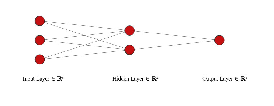
Consider if we had the next layer with just 2 nodes then the linear transformation would look like
\[\mathbf{Z}^{[1]} = \mathbf{X}\mathbf{W}^{[1]}+\mathbf{b}^{[1]}\]where square-bracket superscripts denote the layer under consideration
\[\begin{pmatrix} \text{---} \hspace{-0.2cm} & \mathbf{z}^{[1](1)} & \hspace{-0.2cm} \text{---} \\ \vdots \hspace{-0.2cm} & \vdots & \hspace{-0.2cm} \vdots \\ \text{---} \hspace{-0.2cm} & \mathbf{z}^{[1](m)} & \hspace{-0.2cm} \text{---} \end{pmatrix} = \quad \begin{pmatrix} \text{---} \hspace{-0.2cm} & \mathbf{x}^{(1)} & \hspace{-0.2cm} \text{---} \\ \vdots \hspace{-0.2cm} & \vdots & \hspace{-0.2cm} \vdots \\ \text{---} \hspace{-0.2cm} & \mathbf{x}^{(m)} & \hspace{-0.2cm} \text{---} \end{pmatrix} \begin{pmatrix} \vert & \vert \\ w_1^{[1]} & w_2^{[1]} \\ \vert & \vert \end{pmatrix} + \quad \begin{pmatrix} \text{---} \hspace{-0.2cm} & \mathbf{b}^{[1]} & \hspace{-0.2cm} \text{---} \\ \vdots \hspace{-0.2cm} & \vdots & \hspace{-0.2cm} \vdots \\ \text{---} \hspace{-0.2cm} & \mathbf{b}^{[1]} & \hspace{-0.2cm} \text{---} \end{pmatrix}\]so we had $\mathbf{X}$ being an $m \times k$ matrix, and $\mathbf{W}^{[1]}$ - the matrix of weights for the first layer - is a $k \times n_1$ dimensional matrix if we have $n_1$ nodes in this hidden layer. Here $n_1=2$. If have $m$ training examples we need $m \times n_1$ bias units too. In Python these are in practice “broadcast”.
Imagine the above with a single training example or $m=1$
\[\begin{pmatrix} \text{---} \hspace{-0.2cm} & \mathbf{z}^{[1](1)} & \hspace{-0.2cm} \text{---} \end{pmatrix} = \quad \begin{pmatrix} \text{---} \hspace{-0.2cm} & \mathbf{x}^{(1)} & \hspace{-0.2cm} \text{---} \end{pmatrix} \begin{pmatrix} \vert & \vert \\ w_1^{[1]} & w_2^{[1]} \\ \vert & \vert \end{pmatrix} + \quad \begin{pmatrix} b^{[1]}_1 & b^{[1]}_2 \end{pmatrix}\]We can see that
\[\mathbf{z}^{[1](1)}\]is just a row-vector of shape $1\times n_1$, with each element representing the (linear) output of the neurons in the 1st hidden layer when applied to the first training example.
E.g.
\[\mathbf{Z}^{[1]}_{11}\]would mean the output from the first node, in the first hidden layer after being fed the first training example.
and
\[\mathbf{Z}^{[1]}_{12}\]would be the output from the second node in the first hidden layer, after being fed the first training example.
Going even further, if we reduced the nodes in this layer to just $1$, then we’d have the Perceptron, and the output for a single training example would just be a scalar.
Note: $\mathbf{Z}=\mathbf{X}\mathbf{W}$ could also be written as $\mathbf{Z}^T=\mathbf{W}^T\mathbf{X}^T$ and some people may prefer that convention.
Non-linear step and activation
Next, we would apply an activation function, such as the sigmoid, tanh or ReLu to the outputs from the first hidden layer.
\[\mathbf{A^{[1]}} = \sigma(\mathbf{Z}^{[1]})\]where $\mathbf{A}^{[1]}$ will also be a $m \times n_1$ dimensional matrix.
Subsequent hidden layers
All that happens now is a repeat, instead of feeding the next layer with the design matrix, $\mathbf{X}$, we now feed it $\mathbf{A}^{[1]}$
Linear step
\[\mathbf{Z}^{[2]} = \mathbf{A^{[1]}}\mathbf{W}^{[2]}+\mathbf{b}^{[2]}\]Remember $\mathbf{A}^{[1]}$ is a $m \times n_1$ dimensional matrix, where $m$ is the number of training examples we have and $n_1$ is how many nodes are in the first hidden layer.
This is a bit like we now have $m$ training examples with $n_1$ features each. Each node of the 2nd hidden layer, needs to accept input from each of those $n_1$ features (or outputs from the previous layer if you prefer), meaning each node of the 2nd layer will need $n_1$ weights.
If we have $n_2$ nodes in the 2nd hidden layer, then $\mathbf{W}^{[2]}$ needs to be a $n_1 \times n_2$ dimensional matrix
\[\begin{pmatrix} \text{---} \hspace{-0.2cm} & \mathbf{z}^{[2](1)} & \hspace{-0.2cm} \text{---} \\ \vdots \hspace{-0.2cm} & \vdots & \hspace{-0.2cm} \vdots \\ \text{---} \hspace{-0.2cm} & \mathbf{z}^{[2](m)} & \hspace{-0.2cm} \text{---} \end{pmatrix} = \quad \begin{pmatrix} \text{---} \hspace{-0.2cm} & \mathbf{a}^{[1](1)} & \hspace{-0.2cm} \text{---} \\ \vdots \hspace{-0.2cm} & \vdots & \hspace{-0.2cm} \vdots \\ \text{---} \hspace{-0.2cm} & \mathbf{a}^{[1](m)} & \hspace{-0.2cm} \text{---} \end{pmatrix} \begin{pmatrix} \vert & \dots & \vert \\ w_1^{[2]} & \dots & w_{n_2}^{[2]} \\ \vert & \dots & \vert \end{pmatrix} + \quad \begin{pmatrix} \text{---} \hspace{-0.2cm} & \mathbf{b}^{[2]} & \hspace{-0.2cm} \text{---} \\ \vdots \hspace{-0.2cm} & \vdots & \hspace{-0.2cm} \vdots \\ \text{---} \hspace{-0.2cm} & \mathbf{b}^{[2]} & \hspace{-0.2cm} \text{---} \end{pmatrix}\]Generally the weights matrix of a given layer $l$ will have dimensions
\[\text{dim}(\mathbf{W}^{[l]}) = (n_{l-1}, n_l)\]and the outputs from a given layer (for a single training example) are $1 \times n_{l}$ or $m \times n_{l}$ when considering all $m$ training examples.
Non-linear step and activation
Once again, we would apply an activation function to the outputs from the second hidden layer.
\[\mathbf{A^{[2]}} = \sigma(\mathbf{Z}^{[2]})\]where $\mathbf{A}^{[2]}$ will also be a $m \times n_2$ dimensional matrix.
We’d continue by feeding this into the next hidden layer, and therefore would need $\mathbf{W}^{[3]}$ with dimensions $n_2 \times n_3$.
Generic forward propagation
\[\mathbf{Z}^{[l+1]} = \mathbf{A^{[l]}}\mathbf{W}^{[l+1]}+\mathbf{b}^{[l+1]}\]Which, in terms of elements looks like
\[\mathbf{Z}^{[l+1](i)}_{\quad \quad j} = \sum_{k=1}^{n_l} \mathbf{A}^{[l](i)}_{\quad\, k}\mathbf{W}^{[l+1]}_{kj}+\mathbf{b}^{[l+1](i)}_{\quad\quad\, j}\]Here the column-index $i$ refers to which training example is under consideration and the row index $j$ refers to which node in the layer.
For example
\[\mathbf{Z}^{[3](4)}_{2}\]means the linear output from the 2nd node of the 3rd layer of the NN when it was fed from the 4th training example.
Back propagation
Cost function
Let’s say we have some cost function that we consider as a function of the weights
\[\mathcal{J}(\mathbf{W}) = \frac{1}{m} \sum_{i}^m \mathcal{L^{(i)}}(\mathbf{W})\]and $\mathcal{L_i}$ is the contribution made to that overall cost $\mathcal{J}$ by the ith training example.
We are going to be interested in the derivative of $\mathcal{J}$ with respect to all of our weights and biases (across all layers in the NN). In other words will want to compute
\[\begin{aligned} \frac{\partial \mathcal{J}}{\partial W^{[l]}_{jk}}&=\frac{1}{m}\frac{\partial}{\partial W^{[l]}_{jk}}\left( \sum_{i}^m \mathcal{L^{(i)}}(\mathbf{W}) \right)\\ &=\frac{1}{m} \sum_{i}^m \frac{\partial \mathcal{L^{(i)}}(\mathbf{W}) }{\partial W^{[l]}_{jk}}\quad \text{by linearity of the derivative} \end{aligned}\]for all layers $l$ in the NN, and for all $j, k$ defined by the $1 < j < n_{l-1}$ and $1 < k <, n_{l}$ for a given layer $l$.
We can focus on computing the terms in this sum
\[dW_{jk}^{[l](i)} \stackrel{\text{def}}{=}\frac{\partial \mathcal{L^{(i)}}(\mathbf{W}) }{\partial W^{[l]}_{jk}}\]and then later combine them by summing over the training examples and the $i$ index.
We will also make another definition to help simplify later
\[dZ_{\quad \, p}^{[l](i)} \stackrel{\text{def}}{=}\frac{\partial \mathcal{L^{(i)}}}{\partial Z^{[l](i)}_{\quad \,p}}\]Chain rule
\[\begin{aligned} dW_{jk}^{[l](i)} &\stackrel{\text{def}}{=}\frac{\partial \mathcal{L^{(i)}}(\mathbf{W}) }{\partial W^{[l]}_{jk}}\\ &=\sum_{p=1}^{n_1} \frac{\partial \mathcal{L}^{(i)}}{\partial Z_{\quad \, p}^{[l](i)}}\frac{\partial Z_{\quad \, p}^{[l](i)}}{\partial W^{[l]}_{jk}}\\ &=\sum_{p=1}^{n_1} dZ_{\quad \,p}^{[l](i)} \frac{\partial Z_{\quad \, p}^{[l](i)}}{\partial W^{[l]}_{jk}}\\ &=\sum_{p=1}^{n_1} dZ_{\quad \,p}^{[l](i)} \frac{\partial }{\partial W^{[l]}_{jk}}\left[\sum_{q=1}^{n_{l-1}}A^{[l-1](i)}_{\quad\quad\, q}W^{[l]}_{qp}+\mathbf{b}^{[l](i)}_{\quad\, p} \right]\\ &=\sum_{p=1}^{n_1} dZ_{\quad \,p}^{[l](i)} \left[\sum_{q=1}^{n_{l-1}}A^{[l-1](i)}_{\quad\quad\, q}\frac{\partial W^{[l]}_{qp}}{\partial W^{[l]}_{jk}} \right]\quad \text{linearity of deriv}\\ &=\sum_{p=1}^{n_1} dZ_{\quad \,p}^{[l](i)} \left[\sum_{q=1}^{n_{l-1}}A^{[l-1](i)}_{\quad\quad\, q}\times \delta_{qj}\times \delta_{pk}\right]\\ &= dZ_{\quad \,k}^{[l](i)} A^{[l-1](i)}_{\quad\quad\, j} \end{aligned}\]where here the Kronecker delta
\[\delta_{ij} = \begin{cases} 1, & \text{if } i=j\\ 0, & \text{otherwise} \end{cases}\]and just represents the facts that the derivative of the weights matrix elements are unity if the same element and zero if another element. This allowed us to collapse the sums nicely.
In summary
If we now come back to our actual objective, the derivative of the cost summed over all training examples
\[\begin{aligned} \frac{\partial \mathcal{J}}{\partial W^{[l]}_{jk}}& =\frac{1}{m} \sum_{i}^m dW_{jk}^{[l](i)}\\ &=\frac{1}{m} \sum_{i}^m dZ_{\quad \,k}^{[l](i)} A^{[l-1](i)}_{\quad\quad\, j}\\ &=\frac{1}{m} \sum_{i}^m (A^T)^{[l-1](j)}_{\quad\quad\, i} dZ_{\quad \,\,k}^{[l](i)} \quad \text{taking transpose}\\ &=\frac{1}{m} \left((A^T)^{[l-1]} dZ^{[l]}\right)_{jk}\\ \end{aligned}\]and finally
\[\begin{aligned} \frac{\partial \mathcal{J}}{\partial \mathbf{W}^{[l]}}& =\frac{1}{m} (\mathbf{A}^T)^{[l-1]} \mathbf{dZ}^{[l]}\\ &=\frac{1}{m} (\mathbf{A}^T)^{[l-1]} \frac{\partial \mathcal{L^{(i)}}}{\partial \mathbf{Z}^{[l]}} \end{aligned}\]Recall that $\mathbf{W^{[l]}}$ has dimensions $(n_{l-1}, n_l)$, $\mathbf{A}^{[l-1]}$ has dimensions $(m, n_{l-1})$ and so $\mathbf{A}^T$ has dimensions $(n_{l-1}, m)$, and $\mathbf{Z}^{[l]}$ has dimensions of $(m, n_l)$, so the right hand side has dimensions $(m \times n_{l-1}) \times (m \times n_l)=n_{l-1} \times n_l$, matching what we expected for $\mathbf{W}^{[l]}$.
If I’d have used transposed definitions then I would have ended up with
\[\begin{aligned} \frac{\partial \mathcal{J}}{\partial (\mathbf{W}^T)^{[l]}}& =\frac{1}{m} (\mathbf{dZ}^T)^{[l]} \mathbf{A}^{[l-1]}\\ \end{aligned}\]where $\mathbf{A}$ would be a $m \times n_{l-1}$ matrix with rows representing training examples and each column being the output from the given node in the layer, and $\mathbf{Z}^T$ would be a $n_l \times m$ matrix with columns representing training examples.
Derivative with respect to $Z$
We know how much the cost function changes with $Z$, but we want to know how much it changes with respect to the weights, so we still need to evaluate the terms
\[dZ^{[l](i)}_{\quad \,p} = \frac{\partial \mathcal{L^{(i)}}}{\partial Z^{[l](i)}_{\quad \,p}}\]In order to back-propagate that dependence, it will be helpful to consider the cost’s dependence on the next layer and in turn the next layer’s dependence on this layer.
\[\begin{aligned} dZ^{[l](i)}_{\quad \,p} &= \sum_{q=1}^{n_{l+1}} \frac{\partial \mathcal{L}^{(i)}}{\partial Z^{[l+1](i)}_{\quad\quad\, q}}\frac{\partial Z^{[l+1](i)}_{\quad\quad\, q}}{\partial Z^{[l](i)}_{\quad \,p} }\\ &= \sum_{q=1}^{n_{l+1}} dZ^{[l+1](i)}_{\quad \,q}\frac{\partial Z^{[l+1](i)}_{\quad\quad\, q}}{\partial Z^{[l](i)}_{\quad \,p} }\\ &= \sum_{q=1}^{n_{l+1}} dZ^{[l+1](i)}_{\quad \,q}\frac{\partial}{\partial Z^{[l](i)}_{\quad \,p} }\left[\sum_{r=1}^{n_{l}}A^{[l](i)}_{\quad\, r}W^{[l+1]}_{rq}+\mathbf{b}^{[l+1](i)}_{\quad\quad\, q} \right]\\ &= \sum_{q=1}^{n_{l+1}} dZ^{[l+1](i)}_{\quad \,q}\sum_{r=1}^{n_{l}}W^{[l+1]}_{rq}\frac{\partial A^{[l](i)}_{\quad\, r}}{\partial Z^{[l](i)}_{\quad \,p} }\\ &= \sum_{q=1}^{n_{l+1}} dZ^{[l+1](i)}_{\quad \,q}\sum_{r=1}^{n_{l}}W^{[l+1]}_{rq}\frac{\partial \left(g\left(Z^{[l](i)}_{\quad\, r}\right)\right)}{\partial Z^{[l](i)}_{\quad \,p} }\\ &= \sum_{q=1}^{n_{l+1}} dZ^{[l+1](i)}_{\quad \,q}\sum_{r=1}^{n_{l}}W^{[l+1]}_{rq}\frac{\partial A^{[l](i)}_{\quad\, r}}{\partial Z^{[l](i)}_{\quad \,p} }\\ &= \sum_{q=1}^{n_{l+1}} dZ^{[l+1](i)}_{\quad \,q}\sum_{r=1}^{n_{l}}W^{[l+1]}_{rq}g'\left(Z^{[l](i)}_{\quad\, r}\right)\frac{\partial Z^{[l](i)}_{\quad\, r}}{\partial Z^{[l](i)}_{\quad \,p} }\\ &= \sum_{q=1}^{n_{l+1}} dZ^{[l+1](i)}_{\quad \,q}\sum_{r=1}^{n_{l}}W^{[l+1]}_{rq}g'\left(Z^{[l](i)}_{\quad\, r}\right)\delta_{rp}\\ &= \sum_{q=1}^{n_{l+1}} dZ^{[l+1](i)}_{\quad \,q} W^{[l+1]}_{pq}g'\left(Z^{[l](i)}_{\quad\, p}\right)\\ \end{aligned}\]Here $g$ represents the activation function used after layer $l$.
We have
\[\begin{aligned} dZ^{[l](i)}_{\quad \,p} &= \sum_{q=1}^{n_{l+1}} W^{[l+1]}_{pq}dZ^{[l+1](i)}_{\quad \quad\,q} \times g'\left(Z^{[l](i)}_{\quad\, p}\right)\\ &= \left(\sum_{q=1}^{n_{l+1}} dZ^{[l+1](i)}_{\quad \quad\,q} (W^T)^{[l+1]}_{qp} \right)\times g'\left(Z^{[l](i)}_{\quad\, p}\right)\\ &= \left(dZ^{[l+1]} (W^T)^{[l+1]} \right)^{(i)}_{\quad p} \times g'\left(Z^{[l](i)}_{\quad\, p}\right)\\ \end{aligned}\]This is actually an element-wise multiplication: a given element of the $\mathbf{dZ}^{[l]}$ matrix the product of the same positioned element of the $\mathbf{dZ}^{[l+1]}(\mathbf{W}^T)^{[l+1]}$ matrix, and the same positioned element of the $g’(\mathbf{Z^{[l]}})$ matrix.
We can write it as
\[\begin{aligned} \mathbf{dZ}^{[l]} &= \left(\mathbf{dZ}^{[l+1]} (\mathbf{W}^T)^{[l+1]} \right) \circ g'\left(\mathbf{Z}^{[l]}\right) \end{aligned}\]Where the $\circ$ means element-wise multiplication of the 2 matrices.
Checking the dimensions: $dZ^{[l]}$ has dimensions $m \times n_l$. So $g’(\mathbf{Z}^{[l]})$ also has those dimensions. Next $\mathbf{dZ}^{[l+1]}$ has dimensions $m \times n_{l+1}$ and $(\mathbf{W}^T)^{[l+1]}$ has dimensions of $n_{l+1} \times n_l$, so their matrix product has dimensions of $m \times n_l$. This means the element-wise product is well-defined. Finally we expect $\mathbf{dZ}^{[l]}$ to have the same dimensions as $Z^{[l]}$, i.e. $m \times n_l$, so both sides check out as expected.
Alternative form
Linear backwards
Get the change caused by the current layer’s activations from the change caused by the subsequent layer’s linear outputs
\[\begin{aligned} dA^{[l](i)}_{\quad \,p} &= \sum_{q=1}^{n_{l+1}} \frac{\partial \mathcal{L}^{(i)}}{\partial Z^{[l+1](i)}_{\quad\quad\, q}}\frac{\partial Z^{[l+1](i)}_{\quad\quad\, q}}{\partial A^{[l](i)}_{\quad \,p} }\\ &= \sum_{q=1}^{n_{l+1}} dZ^{[l+1](i)}_{\quad \,q}\frac{\partial Z^{[l+1](i)}_{\quad\quad\, q}}{\partial A^{[l](i)}_{\quad \,p} }\\ &= \sum_{q=1}^{n_{l+1}} dZ^{[l+1](i)}_{\quad \,q}\frac{\partial}{\partial A^{[l](i)}_{\quad \,p} }\left[\sum_{r=1}^{n_{l}}A^{[l](i)}_{\quad\, r}W^{[l+1]}_{rq}+\mathbf{b}^{[l+1](i)}_{\quad\quad\, q} \right]\\ &= \sum_{q=1}^{n_{l+1}} dZ^{[l+1](i)}_{\quad \,q}\sum_{r=1}^{n_{l}}W^{[l+1]}_{rq}\frac{\partial A^{[l](i)}_{\quad\, r}}{\partial A^{[l](i)}_{\quad \,p} }\\ &= \sum_{q=1}^{n_{l+1}} dZ^{[l+1](i)}_{\quad \,q}\sum_{r=1}^{n_{l}}W^{[l+1]}_{rq}\delta_{rp}\\ &= \sum_{q=1}^{n_{l+1}} dZ^{[l+1](i)}_{\quad \,q} W^{[l+1]}_{pq} \end{aligned}\]which can be written
\[\begin{aligned} dA^{[l](i)}_{\quad \,p} &= \sum_{q=1}^{n_{l+1}} W^{[l+1]}_{pq}dZ^{[l+1](i)}_{\quad \quad\,q} \\ &= \left(\sum_{q=1}^{n_{l+1}} dZ^{[l+1](i)}_{\quad \quad\,q} (W^T)^{[l+1]}_{qp} \right)\\ &= \left(dZ^{[l+1]} (W^T)^{[l+1]} \right)^{(i)}_{\quad p} \\ \end{aligned}\]or
\[\mathbf{dA}^{[l]} = \mathbf{dZ}^{[l+1]} (\mathbf{W}^T)^{[l+1]}\]so we have the link between the linear output of the next layer and the activation of the current layer.
Activation backwards
This makes sense given
\[\begin{aligned} \mathbf{dZ}^{[l]} &= \left(\mathbf{dZ}^{[l+1]} (\mathbf{W}^T)^{[l+1]} \right) \circ g'\left(\mathbf{Z}^{[l]}\right) \end{aligned}\]i.e.
\[\mathbf{dZ}^{[l]} = \mathbf{dA}^{[l]} \circ g'\left(\mathbf{Z}^{[l]}\right)\]which is simply telling us that
\[\frac{\partial \mathcal{L}}{\partial \mathbf{Z}}=\frac{\partial \mathcal{L}}{\partial \mathbf{A}} \frac{\partial \mathbf{A}}{\partial \mathbf{Z}}\]Bias terms
\[\begin{aligned} \frac{\partial \mathcal{J}}{\partial \mathbf{b}^{[l]}_{\quad\, p}}&= \frac{1}{m}\sum_{i=1}^m \frac{\partial \mathcal{L^{(i)}}}{\partial \mathbf{b}^{[l]}_{\quad\, p}}\\ &=\frac{1}{m}\sum_{i=1}^m \sum_{k=1}^{n_l}\frac{\partial \mathcal{L^{(i)}}}{\partial \mathbf{Z}^{[l](i)}_{\quad\, k}}\frac{\partial\mathbf{Z}^{[l](i)}_{\quad\, k}}{\partial \mathbf{b}^{[l]}_{\quad\, p}}\\ &=\frac{1}{m}\sum_{i=1}^m \sum_{k=1}^{n_l}\mathbf{dZ}^{[l](i)}_{\quad\,k}\delta_{kp}\\ &=\frac{1}{m}\sum_{i=1}^m \mathbf{dZ}^{[l](i)}_{\quad\,p} \end{aligned}\]which we can denote as
\[\mathbf{db}^{[l]}= \frac{1}{m}\sum_{i=1}^m \mathbf{dZ}^{[l](i)}\]Summary
We have
\[\frac{\partial \mathcal{J}}{\partial \mathbf{W}^{[l]}} =\frac{1}{m} (\mathbf{A}^T)^{[l-1]} \mathbf{dZ}^{[l]}\]and
\[\begin{aligned} \mathbf{dZ}^{[l]} &= \left(\mathbf{dZ}^{[l+1]} (\mathbf{W}^T)^{[l+1]} \right) \circ g'\left(\mathbf{Z}^{[l]}\right) \end{aligned}\]Let’s compose them together
\[\begin{aligned} \frac{\partial \mathcal{J}}{\partial \mathbf{W}^{[l]}}& =\frac{1}{m} (\mathbf{A}^T)^{[l-1]} \mathbf{dZ}^{[l]}\\ &=\frac{1}{m} (\mathbf{A}^T)^{[l-1]}\left[\left(\mathbf{dZ}^{[l+1]} (\mathbf{W}^T)^{[l+1]} \right) \circ g'\left(\mathbf{Z}^{[l]}\right)\right]\\ &=\frac{1}{m} (\mathbf{A}^T)^{[l-1]}\left[\mathbf{dA}^{[l]}\circ g'\left(\mathbf{Z}^{[l]}\right)\right]\\ \end{aligned}\]Once again the dimensions of the square-bracketed part of $m \times n_l$, and the dimensions of $(\mathbf{A}^T)^{[l-1]}$ are $n_{l-1} \times m$ leads to the right-hand side dimensions $n_{l-1}\times n_{l}$, which matches those of $\mathbf{W}^{[1]}$.
Summary of key equations
Note, if we had used the transposed-convention where $\mathbf{\tilde{X}}=\mathbf{X}^T$ is the transpose of the Design matrix (training examples are columns and matrix has dimensions $k \times m$ with $m$ examples and $k$ features), then forward prop would look like
\[\tilde{\mathbf{Z}}=\tilde{\mathbf{W}}\tilde{\mathbf{X}}+\tilde{\mathbf{b}}\]where these quantities are just the transposes
\[\begin{aligned} \tilde{\mathbf{Z}} &\stackrel{\text{def}}{=} \mathbf{Z}^T\\ \tilde{\mathbf{X}} &\stackrel{\text{def}}{=} \mathbf{X}^T\\ \tilde{\mathbf{b}} &\stackrel{\text{def}}{=} \mathbf{b}^T\\ \end{aligned}\]etc
Then we could write the key equations (simply take the transpose of the above equations, ensure to respect $(\mathbf{AB})^T=\mathbf{B}^T\mathbf{A}^T$ and use the new definitions) as
Sometimes these are the equations you will see, but they are totally equivalent, and either is just fine provided you are consistent with notation.
The actual process that the algorithm will do looks like the following
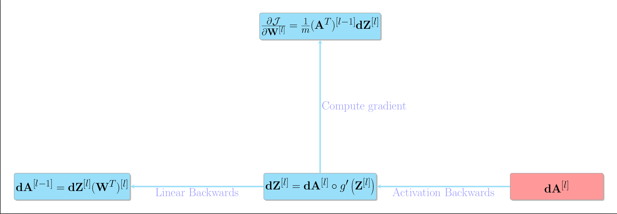
- We are passed $\mathbf{\mathbf{dA}^{[l]}}$, which the subsequent layer computed on its “linear backwards” step
- With this we perform our “activation backwards” step to get $\mathbf{Z}^{[l]}$
- We use that to compute the gradient with respect to this layer’s weights.
- We then compute $\mathbf{\mathbf{dA}^{[l-1]}}$ and pass that back to the previous layer, so it can repeat this process.
Also for efficiency the outputs from each layer $\mathbf{A}$ are usually cached on the forward pass, so they don’t need to be recomputed.
Final layer
$\mathcal{L}_i$ was defined as the contribution to the cost function $\mathcal{J}$ by the ith training example.
For example it may be the cross-entropy loss
\[\mathcal{L}_i = -\log(\mathbf{A^{[L](i)}})\mathbf{Y}^{(i)}\]where for the final layer, $L$, the dimensions of $\mathbf{A^{[L]}}$ are $m \times n_L$, where $n_L$ is the number of nodes in the final layer, which would be the number of classes we wish to classify for example.
Here
\[\mathbf{A}^{[L](i)}\]is a row vector representing the output for the ith training example. The vector $\mathbf{Y}^{i}$ is a column vector (for a fixed $i$)) representing the ground-truth labels for the ith training set. With more training example $\mathbf{Y}$ is a $n_L \times m$ matrix. Representing the true labels for each class for each training example. These are one-hot encoded, i.e. the vector is all zeroes except for the position corresponding to the true class.
Considering if we had just a single training example
\[\mathcal{L} = -\begin{pmatrix} \log (A^{[L]}_1) & \dots & \log(A^{[L]}_{n_L}) \end{pmatrix} \begin{pmatrix} 0\\ \vdots\\ 1\\ \vdots\\ 0 \end{pmatrix}\]which would simply contribute $-\log{A_k^{L}}$. This gives a large penalty when $A_k^{L}$ is near $0$, and gives a small penalty when it is near 1.
The first $\mathbf{dA}^{[L]}$ that we pass backwards will be just
\[\frac{\partial \mathcal{L}}{\partial \mathbf{A}^{[L]}}=-\frac{1}{\mathbf{A}^{[L]}}\mathbf{Y}\]Note that in the binary example with only 2 classes
\[\mathbf{A}^{[L](i)} =\begin{pmatrix}\hat{Y} & 1-\hat{Y}\end{pmatrix}\]Since if we have 2 classes say dog or cat, then if we predict 80% dog, we must predict 20% cat, and
\[\mathbf{Y} = \begin{pmatrix} Y \\ 1-Y \end{pmatrix}\]Since if we have just 2 classes and if $Y=1$ or $Y=0$ then the above specification gives the 2 one-hot encoded vectors necessary.
This gives the familar binary cross entropy:
\[\mathcal{L} = - Y\log{\hat{Y}}-(1-Y)\log{(1-\hat{Y})}\] \[\frac{\partial \mathcal{L}}{\partial Y}=-\frac{Y}{\hat{Y}}+\frac{1-Y}{1-\hat{Y}}\]This will be the first thing we pass backwards to start off the process.


Comments