Vectorized Backprop: Coding it up

In a previous post, I walked through the maths of back-propagation (“backprop”). Here I will go through the implementation in Python (heavily based on Andrew Ng’s course).

I’m going to use the alternative form equations (in the last blog post I denoted those with a tilde, but now I will drop that tilde). This means the design matrix expected is the transpose of the usual. Concretely it is the $k \times m$ dimensional matrix

\[\mathbf{X}=\begin{pmatrix} \vert & \dots & \vert \\ x^{(1)} & \dots & x^{(m)} \\ \vert & \dots & \vert \end{pmatrix}\]

if we have $m$ training examples and $k$ features.

Foward-propagation looks like

\[\mathbf{Z}=\mathbf{W}\mathbf{X}+\mathbf{b}\]

or

\[\begin{pmatrix} \vert & \dots & \vert \\ z^{(1)} & \dots & z^{(m)} \\ \vert & \dots & \vert \end{pmatrix}= \begin{pmatrix} \text{---} \hspace{-0.2cm} & \mathbf{w}^{[1]}_1 & \hspace{-0.2cm} \text{---} \\ \vdots \hspace{-0.2cm} & \vdots & \hspace{-0.2cm} \vdots \\ \text{---} \hspace{-0.2cm} & \mathbf{w}^{[1]}_{n_1} & \hspace{-0.2cm} \text{---} \end{pmatrix} \begin{pmatrix} \vert & \dots & \vert \\ x^{(1)} & \dots & x^{(m)} \\ \vert & \dots & \vert \end{pmatrix} +\quad \begin{pmatrix} \vert & \dots & \vert \\ b^{[1]} & \dots & b^{[1]} \\ \vert & \dots & \vert \end{pmatrix}\]

where the bias is being broadcast.

In this formulation, at each layer the weights matrices have dimensions

\[\text{dim}(\mathbf{W}^{[l]})=n_l \times n_{l-1}\]

the bias matrices have dimensions (after broadcasting over training examples)

\[\text{dim}(\mathbf{b}^{[l]})=n_l \times m\]

and the activations also have this dimension

\[\text{dim}(\mathbf{A}^{[l]})=n_l \times m\]

This leads to the key equations:

\[\begin{aligned} \mathbf{dZ}^{[l]} &=\mathbf{dA}^{[l]}\circ g'\left(\mathbf{Z}^{[l]}\right)\quad \text{activation backwards}\\ \mathbf{dW}^{[l]}& =\frac{1}{m} \left(\mathbf{dZ}\right)^{[l]} \left(\mathbf{A}^{[l-1]}\right)^T \quad \text{compute grad contrib}\\ \mathbf{db}^{[l]}&= \frac{1}{m}\sum_{i=1}^m \mathbf{dZ}^{[l](i)} \quad \text{compute bias grad contrib}\\ \mathbf{dA}^{[l-1]} &= (\mathbf{W}^T)^{[l]} \mathbf{dZ}^{[l]} \quad \text{linear backwards} \end{aligned}\]

Helper functions

First we’ll need some helper functions

Let’s start with the activation functions. Recall that

\[\sigma(z) = \frac{1}{1+e^{-z}}\]

and the rectified-linear unit (ReLu) is defined as

\[f(x) = \begin{cases} x, & \text{if } x>0\\ 0, & \text{otherwise} \end{cases}\]

This implementation returns the original “cached” input as well for reasons of efficiency (we will need to cache those things in the feed-forward for use during the backprop)

import numpy as np

def sigmoid(Z):
    """
    Implements the sigmoid activation in numpy
    
    Arguments:
    Z -- numpy array of any shape
    
    Returns:
    A -- output of sigmoid(z), same shape as Z
    cache -- returns Z as well, useful during backpropagation
    """
    
    A = 1/(1+np.exp(-Z))
    cache = Z
    
    return A, cache

def relu(Z):
    """
    Implement the RELU function.

    Arguments:
    Z -- Output of the linear layer, of any shape

    Returns:
    A -- Post-activation parameter, of the same shape as Z
    cache -- returns Z as well, useful during backpropagation
    """
    
    A = np.maximum(0,Z)
    
    assert(A.shape == Z.shape)
    
    cache = Z 
    return A, cache

We also will need the derivatives to do the “activation backwards” steps.

Recall we had

\[\mathbf{dZ}^{[l]} =\mathbf{dA}^{[l]}\circ g'\left(\mathbf{Z}^{[l]}\right)\]

where this notation means element-wise multiplication. For the sigmoid function its derivative is given by a nice formula

\[\sigma'(x) = \sigma(x)(1-\sigma(x))\]

and for the ReLu activation the derivative is simply

\[f'(x) = \begin{cases} 1, & \text{if } x>0\\ 0, & \text{otherwise} \end{cases}\]

These will be used in the backwards step, and they will take dA passed from the subsequent layer, and also the cache of Z, which was stored during the feed-forward for reasons of efficiency as hopefully will become clearer later.

def relu_backward(dA, cache):
    """
    Implement the backward propagation for a single RELU unit.

    Arguments:
    dA -- post-activation gradient, of any shape
    cache -- 'Z' where we store for computing backward propagation efficiently

    Returns:
    dZ -- Gradient of the cost with respect to Z
    """
    
    Z = cache

    # This is dZ=dA*1
    dZ = np.array(dA, copy=True) # just converting dz to a correct object.
    
    # When z <= 0, you should set dz to 0 as well. 
    dZ[Z <= 0] = 0
    
    assert (dZ.shape == Z.shape)
    
    return dZ

def sigmoid_backward(dA, cache):
    """
    Implement the backward propagation for a single SIGMOID unit.

    Arguments:
    dA -- post-activation gradient, of any shape
    cache -- 'Z' where we store for computing backward propagation efficiently

    Returns:
    dZ -- Gradient of the cost with respect to Z
    """
    
    Z = cache
    
    s = 1/(1+np.exp(-Z))
    
    # dZ = dA * g'
    # dZ = dA * sigmoid(1-sigmoid)
    # Element-wise multiplication
    dZ = dA * s * (1-s)
    
    assert (dZ.shape == Z.shape)
    
    return dZ

Initializing parameters

We will implement a deep NN with $L$ layers. This function will take an array specifying how many nodes in each layer of our NN, e.g. [5,4,3] would mean the input layer has 5 nodes, the hidden layer has 4 nodes and the output layer has 3 nodes. It will randomly initialize the weights and biases matrices that we will need for such a NN and return them in a parameters dictionary.

def initialize_parameters_deep(layer_dims):
    """
    Arguments:
    layer_dims -- python array (list) containing the dimensions of each layer in our network
    
    Returns:
    parameters -- python dictionary containing your parameters "W1", "b1", ..., "WL", "bL":
                    Wl -- weight matrix of shape (layer_dims[l], layer_dims[l-1])
                    bl -- bias vector of shape (layer_dims[l], 1)
    """
    parameters = {} 
    L = len(layer_dims)  # number of layers in the network

    for l in range(1, L):
        # Randomly init n_l x n_{l-1} matrix for weights
        parameters[f'W{l}'] = np.random.randn(layer_dims[l], layer_dims[l-1]) * 0.01
        # Randomly init n_1 x 1 matrix for biases (will be broadcast to n_1 x m)
        parameters[f'b{l}'] = np.zeros((layer_dims[l], 1))
                
    return parameters

This results in the parameters dictionary looking something like

{'W1': [[ 0.01788628,  0.0043651 ,  0.00096497, -0.01863493, -0.00277388],
        [-0.00354759, -0.00082741, -0.00627001, -0.00043818, -0.00477218],
        [-0.01313865,  0.00884622,  0.00881318,  0.01709573,  0.00050034],
        [-0.00404677, -0.0054536 , -0.01546477,  0.00982367, -0.01101068]],
 'W2': [[-0.01185047, -0.0020565 ,  0.01486148,  0.00236716],
        [-0.01023785, -0.00712993,  0.00625245, -0.00160513],
        [-0.00768836, -0.00230031,  0.00745056,  0.01976111]],
 'b1': [[ 0.],
        [ 0.],
        [ 0.],
        [ 0.]],
 'b2': [[ 0.],
        [ 0.],
        [ 0.]]}

Forward propagation

Linear forward

First, implement the linear part. Namely

\[\mathbf{Z}=\mathbf{W}\mathbf{A}+\mathbf{b}\]

where here $\mathbf{A}$ is the activation from the previous layer (or if the first step, then the input data $\mathbf{X}$ as defined above).

def linear_forward(A, W, b):
    """
    Implement the linear part of a layer's forward propagation.

    Arguments:
    A -- activations from previous layer (or input data): (size of previous layer, number of examples)
    W -- weights matrix: numpy array of shape (size of current layer, size of previous layer)
    b -- bias vector, numpy array of shape (size of the current layer, 1)

    Returns:
    Z -- the input of the activation function, also called pre-activation parameter 
    cache -- a python tuple containing "A", "W" and "b" ; stored for computing the backward pass efficiently
    """
    
    Z = np.dot(W, A) + b
    
    assert(Z.shape == (W.shape[0], A.shape[1]))
    cache = (A, W, b)
    
    return Z, cache

Linear activation forward

The next forward step is applying activation to the nodes’ output. We make this step somewhat generic by allowing the user to choose the activation as either sigmoid or ReLu

def linear_activation_forward(A_prev, W, b, activation):
    """
    Implement the forward propagation for the LINEAR->ACTIVATION layer

    Arguments:
    A_prev -- activations from previous layer (or input data): (size of previous layer, number of examples)
    W -- weights matrix: numpy array of shape (size of current layer, size of previous layer)
    b -- bias vector, numpy array of shape (size of the current layer, 1)
    activation -- the activation to be used in this layer, stored as a text string: "sigmoid" or "relu"

    Returns:
    A -- the output of the activation function, also called the post-activation value 
    cache -- a python tuple containing "linear_cache" and "activation_cache";
             stored for computing the backward pass efficiently
    """
    
    if activation == "sigmoid":
        Z, linear_cache = linear_forward(A_prev, W, b)
        A, activation_cache = sigmoid(Z)
    
    elif activation == "relu":
        Z, linear_cache = linear_forward(A_prev, W, b)
        A, activation_cache = relu(Z)
    
    assert (A.shape == (W.shape[0], A_prev.shape[1]))
    cache = (linear_cache, activation_cache)

    return A, cache

L layers

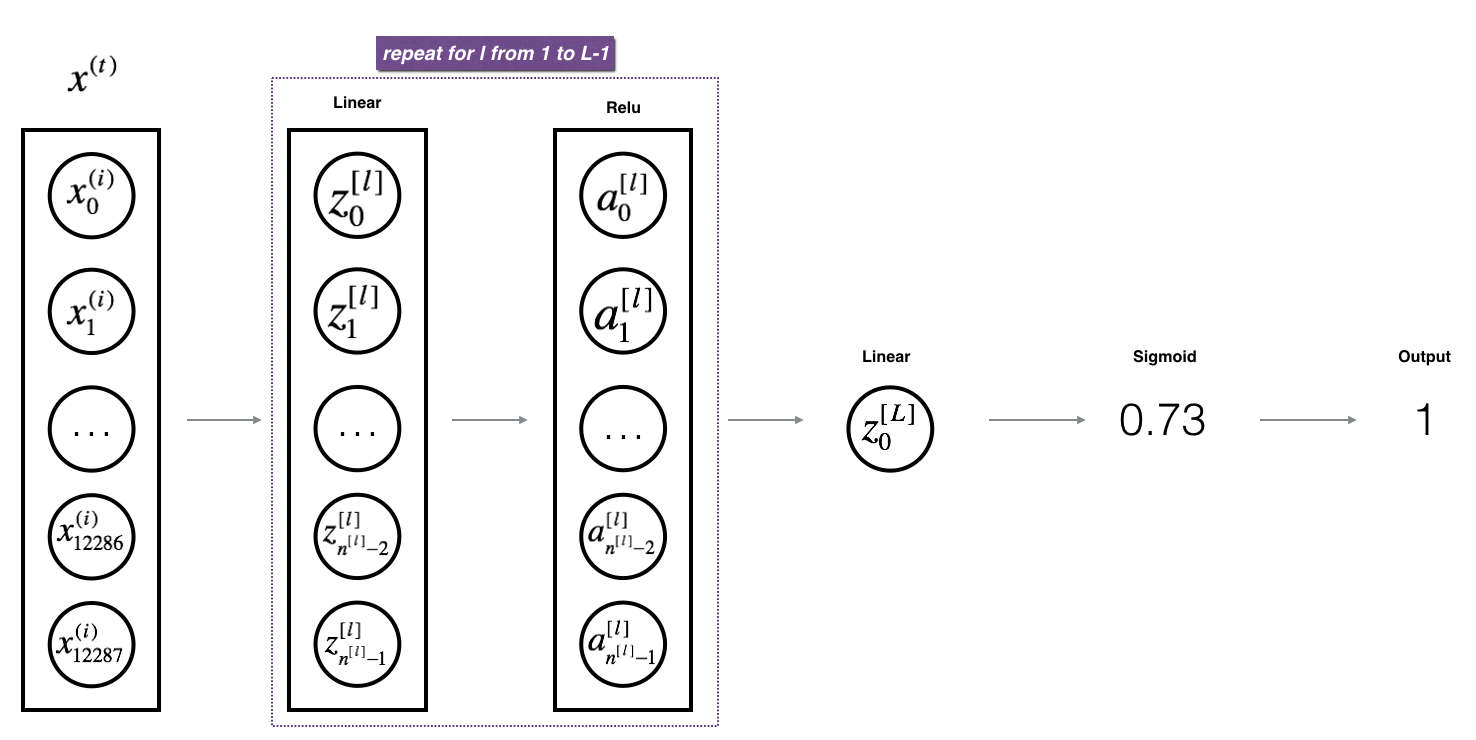
For this NN we want to have L-1 layers that are “Linear + ReLu” and the output layer to be “Linear + Sigmoid”. The want the final layer to be sigmoid so that we can get predictions that represent probabilities for each of our classes with something like softmax.

def L_model_forward(X, parameters):
    """
    Implement forward propagation for the [LINEAR->RELU]*(L-1)->LINEAR->SIGMOID computation
    
    Arguments:
    X -- data, numpy array of shape (input size, number of examples)
    parameters -- output of initialize_parameters_deep()
    
    Returns:
    AL -- last post-activation value
    caches -- list of caches containing:
                every cache of linear_activation_forward() (there are L-1 of them, indexed from 0 to L-1)
    """

    # Record the caches for later efficiency
    caches = []

    # Initial input is the design matrix transposed, X
    A = X

    # number of layers in the neural network (has 2L keys, weights+biases each layer)
    L = len(parameters) // 2  
    
    # [LINEAR -> RELU]*(L-1) layers
    for l in range(1, L):
        A_prev = A 
        A, cache = linear_activation_forward(A_prev, parameters[f"W{l}"], parameters[f"b{l}"], "relu")
        caches.append(cache)
    
    # Output layer LINEAR -> SIGMOID. 
    AL, cache = linear_activation_forward(A, parameters[f"W{L}"], parameters[f"b{L}"], "sigmoid")
    caches.append(cache)
    
    # We expect the final layer to be (1, m) row vector of predictions (1 per training example)
    # If binary classification
    assert(AL.shape == (1, X.shape[1]))
            
    return AL, caches

Cost function

In this simple example, we just implement a simple binary classification cost function.

We expect the final output to be a $1 \times m$ row vector - a prediction $\hat{Y}^{(i)}=A^{[L] (i)}$ for each training example. The ground truth labels for each training example is the $1 \times m$ row vector $\mathbf{Y}$ with a $1$ or $0$ at each position.

The binary cross-entropy is

\[\mathcal{L} = -\frac{1}{m} \sum\limits_{i = 1}^{m} \mathbf{Y}^{(i)}\log\mathbf{\hat{Y}}^{(i)} + (1-\mathbf{Y}^{(i)})\log\left(1- \mathbf{\hat{Y}}^{(i)}\right) \]

In vectorized form this looks like

\[\mathcal{L} = - \frac{1}{m} \mathbf{Y}\left(\log{\mathbf{\hat{Y}}}\right)^T-(\mathbf{1}-\mathbf{Y})\left(\log{(\mathbf{1}-\hat{\mathbf{Y}})}\right)^T\]

def compute_cost(AL, Y):
    """
    Implement the cost function defined by equation

    Arguments:
    AL -- probability vector corresponding to your label predictions, shape (1, number of examples)
    Y -- true "label" vector (for example: containing 0 if non-cat, 1 if cat), shape (1, number of examples)

    Returns:
    cost -- cross-entropy cost
    """
    # How many training examples
    m = Y.shape[1]

    # Compute loss from AL and Y.
    cost = (-1/m)*(np.dot(Y, np.log(AL).T)+np.dot((1-Y), np.log(1-AL).T))
    
    # Get the right shape, e.g. squeeze turns [[1]] to 1
    cost = np.squeeze(cost)    

    return cost

Backward propagation (backprop)

Linear backwards

We implement this part of the key equations

\[\begin{aligned} \mathbf{dW}^{[l]}& =\frac{1}{m} \left(\mathbf{dZ}\right)^{[l]} \left(\mathbf{A}^{[l-1]}\right)^T \quad \text{compute grad contrib}\\ \mathbf{db}^{[l]}&= \frac{1}{m}\sum_{i=1}^m \mathbf{dZ}^{[l](i)} \quad \text{compute bias grad contrib}\\ \mathbf{dA}^{[l-1]} &= (\mathbf{W}^T)^{[l]} \mathbf{dZ}^{[l]} \quad \text{linear backwards} \end{aligned}\]

This step computes the $\mathbf{dA}$ that we will pass backwards to the previous layer. It needs the linear gradient $\mathbf{dZ}$ of the current layer (which we will soon compute in the “activation backwards” step) and the current layer weights and previous layer activation outputs (both of which we handily cached during forward propagation).

It also computes the gradient contributions of this layer, $\mathbf{dW}$ and $\mathbf{db}$.

def linear_backward(dZ, cache):
    """
    Implement the linear portion of backward propagation for a single layer (layer l)

    Arguments:
    dZ -- Gradient of the cost with respect to the linear output (of current layer l)
    cache -- tuple of values (A_prev, W, b) coming from the forward propagation in the current layer

    Returns:
    dA_prev -- Gradient of the cost with respect to the activation (of the previous layer l-1), same shape as A_prev
    dW -- Gradient of the cost with respect to W (current layer l), same shape as W
    db -- Gradient of the cost with respect to b (current layer l), same shape as b
    """

    # Grab from the cache, since we are going to need the current layer weights
    A_prev, W, b = cache

    # The activation matrices A should have dimension n_l x m
    m = A_prev.shape[1]

    # Compute dA to pass back to previous layer 
    dA_prev = np.dot(W.T, dZ)

    # Gradient contributions of this layer
    # dim(dZ)=n_l x m, dim(A_prev)=n_{l-1} x m
    # dZ.A_prev^T has dims n_l x n_{l-1}
    dW = (1/m)*np.dot(dZ, A_prev.T)

    # dZ has dims of n_l x m and db has dims like b, i.e. n_l x 1 (before the broadcasting)
    # so we need to sum over training examples -> axis=1 (across columns)
    # https://numpy.org/doc/stable/reference/generated/numpy.sum.html
    db = 1/m*(np.sum(dZ, axis=1, keepdims=True))

    
    # Dimensional sanity checks (grads have sample dims as originals)
    assert (dA_prev.shape == A_prev.shape)
    assert (dW.shape == W.shape)
    assert (db.shape == b.shape)
    
    return dA_prev, dW, db

Linear and Activation backwards

The linear layer needed $\mathbf{dZ}$ as input. In this step we compute it from the post-activation gradient $\mathbf{dA}$ that the subsequent layer would have passed back to us. We already implemented some helper functions to do that, so this function just composes the linear backwards and activation backwards steps.

 def linear_activation_backward(dA, cache, activation):
    """
    Implement the backward propagation for the LINEAR->ACTIVATION layer.
    
    Arguments:
    dA -- post-activation gradient for current layer l 
    cache -- tuple of values (linear_cache, activation_cache) we store for computing backward propagation efficiently
    activation -- the activation to be used in this layer, stored as a text string: "sigmoid" or "relu"
    
    Returns:
    dA_prev -- Gradient of the cost with respect to the activation (of the previous layer l-1), same shape as A_prev
    dW -- Gradient of the cost with respect to W (current layer l), same shape as W
    db -- Gradient of the cost with respect to b (current layer l), same shape as b
    """
    # Linear cache is the A_prev, W, b, activation cache is the Z    
    linear_cache, activation_cache = cache
    
    if activation == "relu":
        dZ = relu_backward(dA, activation_cache)
        dA_prev, dW, db = linear_backward(dZ, linear_cache)
        
    elif activation == "sigmoid":
        dZ = sigmoid_backward(dA, activation_cache)
        dA_prev, dW, db = linear_backward(dZ, linear_cache)
    
    return dA_prev, dW, db

L layers backwards

\[\frac{\partial \mathcal{L}}{\partial Y}=-\frac{Y}{\hat{Y}}+\frac{1-Y}{1-\hat{Y}}\]

def L_model_backward(AL, Y, caches):
    """
    Implement the backward propagation for the [LINEAR->RELU] * (L-1) -> LINEAR -> SIGMOID group
    
    Arguments:
    AL -- probability vector, output of the forward propagation (L_model_forward())
    Y -- true "label" vector (containing 0 if non-cat, 1 if cat)
    caches -- list of caches containing:
                every cache of linear_activation_forward() with "relu" (it's caches[l], for l in range(L-1) i.e l = 0...L-2)
                the cache of linear_activation_forward() with "sigmoid" (it's caches[L-1])
    
    Returns:
    grads -- A dictionary with the gradients
             grads["dA" + str(l)] = ... 
             grads["dW" + str(l)] = ...
             grads["db" + str(l)] = ... 
    """
    grads = {}
    L = len(caches) # the number of layers

    # AL has shape (1 x m) - prediction per training example
    m = AL.shape[1]

    # Ensure the ground truth labels are also shape (1 x m) [not m x 1]
    Y = Y.reshape(AL.shape) 
    
    # Initializing the backpropagation: derivative of cost with respect to AL
    dAL = - (np.divide(Y, AL) - np.divide(1 - Y, 1 - AL)) 
    
    # Lth layer (SIGMOID -> LINEAR) gradients. 
    current_cache = caches[L-1]  
    # Remember this spits out the dA for the previous layer (to pass back) and the gradient contribs
    # for the current layer
    grads[f"dA{L-1}"], grads[f"dW{L}"], grads[f"db{L}"] = linear_activation_backward(dAL, current_cache, "sigmoid")
    
    # Loop from l=L-2 to l=0   e.g. list(reversed(range(5-1))) = [3, 2, 1, 0]
    for l in reversed(range(L-1)):
        # lth layer: (RELU -> LINEAR) gradients.
        current_cache = caches[l]
        grads[f"dA{l}"], grads[f"dW{l+1}"], grads[f"db{l+1}"] = linear_activation_backward(grads[f"dA{l+1}"], current_cache, "relu")

    return grads

Update parameters

All that is left to do now is update the weights and biases

\[\begin{aligned} W^{[l]} &= W^{[l]} - \alpha \text{ } dW^{[l]} \\ b^{[l]} &= b^{[l]} - \alpha \text{ } db^{[l]} \end{aligned}\]

where here $\alpha$ is the learning rate hyperparameter.

def update_parameters(parameters, grads, learning_rate):
    """
    Update parameters using gradient descent
    
    Arguments:
    parameters -- python dictionary containing your parameters 
    grads -- python dictionary containing your gradients, output of L_model_backward
    
    Returns:
    parameters -- python dictionary containing your updated parameters 
                  parameters["W" + str(l)] = ... 
                  parameters["b" + str(l)] = ...
    """
    
    L = len(parameters)// 2 # number of layers in the neural network (since each layer has weights+bias)

    # Update rule for each parameter. Use a for loop.
    for l in range(L):
        parameters[f"W{l+1}"] = parameters[f"W{l+1}"] - (learning_rate*grads[f"dW{l+1}"])
        parameters[f"b{l+1}"] = parameters[f"b{l+1}"] - (learning_rate*grads[f"db{l+1}"])
    return parameters

Putting it all together

def L_layer_model(X, Y, layers_dims, learning_rate = 0.0075, num_iterations = 3000, print_cost=False):
    """
    Implements a L-layer neural network: [LINEAR->RELU]*(L-1)->LINEAR->SIGMOID.
    
    Arguments:
    X -- data, numpy array of shape (num_px * num_px * 3, number of examples)
    Y -- true "label" vector (containing 0 if cat, 1 if non-cat), of shape (1, number of examples)
    layers_dims -- list containing the input size and each layer size, of length (number of layers + 1).
    learning_rate -- learning rate of the gradient descent update rule
    num_iterations -- number of iterations of the optimization loop
    print_cost -- if True, it prints the cost every 100 steps
    
    Returns:
    parameters -- parameters learnt by the model. They can then be used to predict.
    """

    costs = []   # keep track of cost
    
    # Parameters initialization
    parameters = initialize_parameters_deep(layers_dims)
    
    # Loop (gradient descent)
    for i in range(0, num_iterations):

        # Forward propagation: [LINEAR -> RELU]*(L-1) -> LINEAR -> SIGMOID.
        AL, caches = L_model_forward(X, parameters)
        
        # Compute cost.
        cost = compute_cost(AL, Y)
    
        # Backward propagation.
        grads = L_model_backward(AL, Y, caches)
 
        # Update parameters.
        parameters = update_parameters(parameters, grads, learning_rate)
                
        # Print the cost every 100 training example
        if print_cost and i % 100 == 0:
            print ("Cost after iteration %i: %f" %(i, cost))
        if print_cost and i % 100 == 0:
            costs.append(cost)
            
    # plot the cost
    plt.plot(np.squeeze(costs))
    plt.ylabel('cost')
    plt.xlabel('iterations (per hundreds)')
    plt.title("Learning rate =" + str(learning_rate))
    plt.show()
    
    return parameters

To run this model, we define the layer dimensions for the network

layers_dims = [12288, 20, 7, 5, 1] #  e,g 4-layer model
parameters = L_layer_model(train_x, train_y, layers_dims, num_iterations = 2500, print_cost = True)

Testing it

To test it we could use a simple binary classification problem such as the Sklearn Breast Cancer Dataset.

This dataset has data with 30 features used to detect whether a breast tumour is malignant or benign, such as the “mean radius”.

from sklearn.datasets import load_breast_cancer
from sklearn.model_selection import train_test_split
X, y = load_breast_cancer(return_X_y=True)
X_train, X_test, y_train, y_test = train_test_split(X, y, random_state=0)

The shape of X_train.shape is (426, 30) i.e. this is $m \times k$ and we need $k \times m$, so we will need to transpose. Moreover y_train.shape is (426,) and we’ll need to reshape that to (1, 426).

X_train_T = X_train.T   # Our formulation expects transpose of design matrix
X_test_T = X_test.T
y_train = y_train.reshape(1, -1)  # We need 1 x m
y_test = y_test.reshape(1, -1)  # We need 1 x m

Let’s try a 4-layer NN

layers_dims = [30, 20, 7, 5, 1] #  4-layer model

Notice the input layer is 30 since our data has 30 features. The first hidden layer has 20 nodes, the next 7, the next 5 and finally the output layer is 1 corresponding to our prediction of malignant or benign.

Training the model

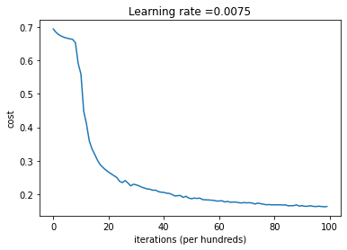
parameters = L_layer_model(X_train_T, y_train, layers_dims, num_iterations = 10000, print_cost = True)

Cost after iteration 0: 0.693144
Cost after iteration 100: 0.683078
Cost after iteration 200: 0.676150
Cost after iteration 300: 0.671366
Cost after iteration 400: 0.668043
Cost after iteration 500: 0.665694
Cost after iteration 600: 0.663928
Cost after iteration 700: 0.662127
Cost after iteration 800: 0.652339
Cost after iteration 900: 0.590585
Cost after iteration 1000: 0.558723
Cost after iteration 1100: 0.448147
Cost after iteration 1200: 0.410654
Cost after iteration 1300: 0.360289
Cost after iteration 1400: 0.335892
Cost after iteration 1500: 0.319279
Cost after iteration 1600: 0.301837
Cost after iteration 1700: 0.288383
Cost after iteration 1800: 0.280121
Cost after iteration 1900: 0.272764
.
.
.
Cost after iteration 8800: 0.168956
Cost after iteration 8900: 0.165194
Cost after iteration 9000: 0.166604
Cost after iteration 9100: 0.164738
Cost after iteration 9200: 0.164705
Cost after iteration 9300: 0.166488
Cost after iteration 9400: 0.164538
Cost after iteration 9500: 0.163890
Cost after iteration 9600: 0.165013
Cost after iteration 9700: 0.164089
Cost after iteration 9800: 0.163319
Cost after iteration 9900: 0.164118

Testing the accuracy

def predict(X, y, parameters):
    """
    This function is used to predict the results of a  L-layer neural network.
    
    Arguments:
    X -- data set of examples you would like to label
    parameters -- parameters of the trained model
    
    Returns:
    p -- predictions for the given dataset X
    """
    
    m = X.shape[1]
    n = len(parameters) // 2 # number of layers in the neural network
    p = np.zeros((1, m))
    
    # Forward propagation
    probas, caches = L_model_forward(X, parameters)

    
    # convert probas to 0/1 predictions
    for i in range(0, probas.shape[1]):
        if probas[0,i] > 0.5:
            p[0, i] = 1
        else:
            p[0, i] = 0
    

    print("Accuracy: "  + str(np.sum((p == y)/m)))
        
    return p

First let’s check the accuracy on the training set

pred_train = predict(X_train_T, y_train, parameters)
Accuracy: 0.9342723004694834

Not bad. What about the test set?

pred_test = predict(X_test_T, y_test, parameters)
Accuracy: 0.937062937062937

So seems our model is doing quite well!

Here is a link to a Google Colab containing the above code.