Forecasting the price of bitcoin using an LSTM

I’m sure that every developer who has learned a little bit of ML dreams of applying this to the stock market and getting rich. At first glance RNNs and LSTMs seem perfect tools for the job. Something tells me it’s not going to be that easy, but it can be fun to try and this post will do that.

Getting the data

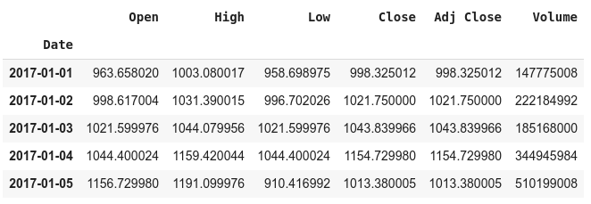
We will use the yfinance package to get the historic Bitcoin price data

!pip install yfinance
import yfinance as yf
BTC_price_data = yf.download('BTC-USD','2017-01-01', time.strftime('%Y-%m-%d'))

BTC_price_data.head()

We will try to predict the closing prices

np_data = BTC_price_data.Close.to_numpy()

Training and test sets

It’s important that we test our model on unseen data, so we split the data into a training set and a test set. The standard amount is 80:20. You may also want to try this with a threeway training-validation-test split. But for now we will keep it simple.

def split_data(data, training_size=0.8):
  return data[:int(training_size*len(data))], data[in(training_size*len(data)):]

training_data, test_data = split_data(np_data)

Windowing

The basic idea is that we will feed into our network closing prices for some previous days (e.g. previous 5 days for example) and we want it predict the next day’s closing price.

We could vary the length of the window of previous days that we use as features.

As an example let’s say we had the time series with values [1, 2, 3, 4, 5, 6], and we had a window length of 2, then our training examples are

[1, 2] -> 3
[2, 3] -> 4
[3, 4] -> 5
[4, 5] -> 6

Returns

The return also known as percentage return, raw return, linear return or simple return is defined as

\[\begin{aligned} r&=\frac{p_t - p_{t-1}}{p_{t-1}}\\ r&=\Bigg(\frac{p_t}{p_{t-1}}\Bigg)-1 \end{aligned}\]

where $p_t$ is the price of the stock at a given time.

For various reasons, it makes more sense to look at returns rather than prices.

The next thing we need to do is normalize our training examples relative to the initial value of the series at the start of the window. So for example [1, 2] - > 3 would be normalized as [0, 1] -> 2.

def normalize_window(w):
    return (w/w[0]) -1

We shuffle the data to avoid bias. Finally we split the example into input/target, e.g. [[1, 2], [3]], and we batch it into batches of batch_size

# Check TF 2.0
import tensorflow as tf
print(tf.__version__)

from keras.models import Sequential
from keras.layers import Activation, Dense
from keras.layers import LSTM
from keras.layers import Dropout, Conv1D

import matplotlib.pyplot as plt
import numpy as np


def windowed_dataset(series):
    # Initially the data is (1188,) expand dims to TensorShape([1188, 1])
    series = tf.expand_dims(series, axis=-1)

    # https://www.tensorflow.org/api_docs/python/tf/data/Dataset
    # will be an iterable of tf.Tensor([998.325], shape=(1,), dtype=float32),...
    ds = tf.data.Dataset.from_tensor_slices(series)
    
    # https://stackoverflow.com/questions/55429307/how-to-use-windows-created-by-the-dataset-window-method-in-tensorflow-2-0
    # The +1 accounts for the label too. Create a bunch of windows over our series
    # If we started with ds = tf.data.Dataset.from_tensor_slices([1,2,3,4,5])
    # then ds = ds.window(3, shift=1, drop_remainder=False) would lead
    # to [1,2,3], [2, 3, 4], [3, 4, 5], [4, 5], [5] whereas 
    # drop_remainder=True) => [1,2,3], [2, 3, 4], [3, 4, 5]
    ds = ds.window(window_len + 1, shift=1, drop_remainder=True)
    # Maps map_func across this dataset and flattens the result
    ds = ds.flat_map(lambda w: w.batch(window_len + 1))

    def normalize_window(w):
      return (w/w[0]) -1

    ds = ds.map(normalize_window)

    # randomize order 
    ds = ds.shuffle(shuffle_buffer)
    
    # Collect the inputs and the label
    ds = ds.map(lambda w: (w[:-1], w[-1]))

    return ds.batch(batch_size).prefetch(1)
model_training_data = windowed_dataset(training_data)

The model with Keras

def build_model(output_size, neurons, activ_func=activation_function, dropout=dropout, loss=loss, optimizer=optimizer):
  model = tf.keras.models.Sequential([
  tf.keras.layers.Conv1D(filters=25, kernel_size=5,
                      strides=1, padding="causal",
                      activation="relu",
                      input_shape=[None, 1]),
  # tf.keras.layers.LSTM(neurons, input_shape=[None, None, 1], return_sequences=True, activation=activ_func),
  tf.keras.layers.LSTM(neurons, return_sequences=True, activation=activ_func),
  tf.keras.layers.Dropout(dropout),
  tf.keras.layers.LSTM(neurons, return_sequences=True, activation=activ_func),
  tf.keras.layers.Dropout(dropout),
  tf.keras.layers.LSTM(neurons, return_sequences=True, activation=activ_func),
  tf.keras.layers.Dropout(dropout),
  tf.keras.layers.LSTM(neurons, return_sequences=False, activation=activ_func),
  tf.keras.layers.Dropout(dropout),
  tf.keras.layers.Dense(units=output_size, activation=activ_func),
  ])
  model.compile(loss=loss, optimizer=optimizer, metrics=['mae'])
  model.summary()
  return model

Build the model

# Clean up the memory
tf.keras.backend.clear_session()
btc_model = build_model(output_size=1, neurons=neurons)

Fit the model

btc_history = btc_model.fit(model_training_data, epochs=epochs, batch_size=batch_size, verbose=1)

Forecast

def model_forecast(model, series):
    # Initially the data is (N,) expand dims to TensorShape([N, 1])
    series = tf.expand_dims(series, axis=-1)

    # Now we just use window_len not +1, because we just want inputs not label, and we predict label
    ds = tf.data.Dataset.from_tensor_slices(series)
    ds = ds.window(window_len, shift=1, drop_remainder=True)
    ds = ds.flat_map(lambda w: w.batch(window_len))

    def normalize_window(w):
      return w/w[0] -1

    ds = ds.map(normalize_window)

    ds = ds.batch(32).prefetch(1)

    return model.predict(ds)