

Coin flip power analysis
Deciding if a coin is fair
We can have a statistical model for single flip of the coin: $({0, 1}, {\sim\text{Ber}(p)}_{p \in (0, 1)})$ (means the result is either 0 (tails) or 1 (heads) and the distribution is just a Bernoulli with prob $p$ of $1$ and $(1-p)$ of $0$)
Then the null and alternative hypotheses are
- $H_0$: coin is fair with probability 50% of heads and 50% of tails. $p=0.5$, i.e. $\Theta_0 = {0.5}$
- $H_1$: coin is not fair with $p\neq 0.5$, i.e. $\Theta_1 = (0, 1)\setminus{0.5}$ (all probs on the closed interval excluding 0.5)
Test statistic
We use the test statistic
\[T_n = \sqrt{n}\frac{|\bar{X}_n - 1/2|}{\sqrt{1/2(1-1/2)}}=2\sqrt{n}|\bar{X}_n-1/2|\]Why do we choose this as our test statistics? Well, if $X_j \sim \text{Ber}(p)$, then
\[\begin{aligned} \text{var}(\bar{X}_n)&=\text{var}\left(\frac{X_1 + \dots + X_n}{n}\right)\\ &=\frac{1}{n^2}\text{var}(X_1+\dots+X_n)\\ &=\frac{n}{n^2}\text{var}(X_1)\\ &=\frac{1}{n}p(1-p) \end{aligned}\]where the first step follows from $\text{var}(aX)=a^2\text{var}{X}$, the second step follows from the fact that the $X_j \stackrel{iid}{\sim} \text{Ber}(p)$, i.e. they are all assumed independent, identically distributed random variables with the same mean and variance, plus linearity of variance for independent random variables, $\text{var}(X+Y)=\text{var}(X)+\text{var}(Y)$, if $X, Y$ are independent.Finally we use the fact that the variance of a Bernoulli is $p(1-p)$ as can be easily demonstrated.
Variance of a Bernoulli
\[\text{var}[X] = \text{E}(X^2) - (\text{E}(X))^2\]The expectation is just
\[\text{E}(X) = p\times 1 + (1-p)\times 0 = p\]The second moment is
\[\text{E}(X^2) = p\times 1^2 + (1-p)\times 0^2 = p\]Therefore
\[\text{var}[X] = p-p^2=p(1-p)\]CLT
The CLT tells us that the sum will be normally distributed as $n \to \infty$. Iff we want a standard normal $\sim \mathcal{N}(0, 1)$ then we need to subtract the mean ($p$) and the divide by the standard deviation. It’s easy to verify that the variance of this demeaned and rescaled random variable will be 1 (See Introduction to Probability- Dimitri P. Bertsekas (Author), John N. Tsitsiklis, ch5, p274 for example)
If we assume the coin is fair, $p=0.5$, then as $n\to \infty$ we’d expect
\[2\sqrt{n}(\bar{X}_n - 1/2) \xrightarrow[n \to \infty]{(d)} \mathcal{N}(0, 1)\]Test
We design a test
\[\psi_{\alpha} = \mathbb{1}(T_n > c_{\alpha})\]i.e. $\psi_{\alpha}=1$ when we reject the null-hypothesis, and $\psi_{\alpha}=0$ when we fail to reject it (never “accept” it as such, only either reject or fail to reject).
Errors
Type 1 error
This happens when we reject the null and we shouldn’t have, in other words if we have $\theta \in \Theta_0$ (in our case $p=1/2$) and $\psi_{\alpha}=1$, or the coin is fair, but we reject it being so. The “level” of the test $\alpha$ is the largest probability of rejecting the null hypothesis over $\Theta_0$:
\[\lim_{n\to\infty} P_{1/2}(\psi=1) \le \alpha\]If $p=1/2$, then by the CLT then the probability of a type 1 error goes as if we choose $C=q_{\alpha/2}$
\[P(\psi=1) = P\left(2\sqrt{n}|\bar{X}_n-1/2| > q_{\alpha/2}\right) \to \alpha\]where $q_{\alpha/2}$ is the $1-\alpha/2$ quantile. We can therefore limit our type 1 error and get a level $\alpha$ if we choose $C$ like this.
Type 2 error
\[\begin{aligned} &\beta_{\psi_n}: \Theta_1 \to \mathbb{R}\\ &\theta \mapsto P_{\theta}(\psi_n=0) \end{aligned}\]In words, this is saying that if the alternative hypothesis is true ($\theta \in \Theta_1$ or in our case $p\ne 1/2$, coin not fair), what is the probability that we fail to reject the null hypothesis, and therefore commit a type 2 error. E.g the coin has bias 0.6 but we fail to reject the null hypothesis that the coin is fair.
Well if we have a fair coin we reject if
\[\begin{aligned} &2\sqrt{n}|\bar{X}_n-1/2| > q_{\alpha/2}\\ &=|\bar{X}_n-1/2| > \frac{q_{\alpha/2}}{2\sqrt{n}}\\ \end{aligned}\]which means our rejection region is
\[\bar{X}_n > \frac{1}{2}+\frac{q_{\alpha/2}}{2\sqrt{n}}\]or
\[\bar{X}_n < \frac{1}{2}-\frac{q_{\alpha/2}}{2\sqrt{n}}\]Python
from scipy.stats import norm
import numpy as np

# Get the q alpha/2
alpha = 0.05 # level
p = 0.5 # fair coin
n = 100 # how many flips
q = norm.ppf(1-alpha/2)
print(f'The value of q is {q:.2f} when alpha is {alpha}')


lower_r = 0.5-q/(2*np.sqrt(n))
upper_r = 0.5+q/(2*np.sqrt(n))

print(f'The rejection region is less than {lower_r:.2f} or above {upper_r:.2f}')
print(f'{(1-alpha)*100} % of the time we get a count of heads out of {n} flips between {n*lower_r:.2f} and {n*upper_r:.2f} if n={n}')
Running this script tells me that if $n=100$ and $\alpha=0.05$, with a fair coin we’d reject the null hypothesis (erroneously, type 1 error) if we had less than 40 heads or more than 60 heads. Our rejection rejection, $R_{\psi_n}$ is therefore less than 40 or above 60.
What is the probability that we reject the null hypothesis when $p\ne 0.5$?
This is known as the “statistical power” of the test
The power of the test is formally defined as
\[\pi_{\psi_n} = \inf_{\theta \in \Theta_1} (1-\beta_{\theta_{\psi_n}}(\theta))\]Over the space of parameters defining the alternative hypothesis (where we should be rejecting the null), what is our “smallest” chance of rejecting the null….our smallest chance of scientific discovery etc…
For the coin I want to plot the probability of rejecting the null over $p\ne 0.5$
We reject on the right if
\[\begin{aligned} &P\left(\bar{X_n} > \frac{1}{2} + \frac{q_{\alpha/2}}{2\sqrt{n}}\right)\\ &=P\left(\bar{X_n} - p > \frac{1}{2} - p + \frac{q_{\alpha/2}}{2\sqrt{n}}\right)\\ &=P\Bigg(2\sqrt{n}(\bar{X_n} - p) > 2\sqrt{n}\left(1/2 - p\right) + q_{\alpha/2}\Bigg)\\ \end{aligned}\]where here we are now considering the true param being $p\ne1/2$.
$2\sqrt{n}(\bar{X_n} - p) \sim \mathcal{N}(0, 1)$ if the true param is $p$. So the probability goes as
\[1-\Phi\Big(q_{\alpha/2} + 2\sqrt{n}\left(1/2 - p\right) \Big)\]Notice if $p>1/2$ then this would decrease the $q$ decreasing the CDF and increasing the probability of rejection…But if $p=1/2$ there’d be no change.
Similarly, reject on the left if
\[\begin{aligned} &P\left(\bar{X_n} < \frac{1}{2} - \frac{q_{\alpha/2}}{2\sqrt{n}}\right)\\ &=P\left(\bar{X_n} - p < \frac{1}{2} - p - \frac{q_{\alpha/2}}{2\sqrt{n}}\right)\\ &=P\Bigg(2\sqrt{n}(\bar{X_n} - p) < 2\sqrt{n}\left(1/2 - p\right) - q_{\alpha/2}\Bigg)\\ \end{aligned}\]where here we are now considering the true param being $p\ne1/2$.
$2\sqrt{n}(\bar{X_n} - p) \sim \mathcal{N}(0, 1)$ if the true param is $p$. So the probability goes as
\[\Phi\Big(-q_{\alpha/2} + 2\sqrt{n}\left(1/2 - p\right) \Big)\]The total probability of rejection is therefore
\[1-\Phi\Big(q_{\alpha/2} + 2\sqrt{n}\left(1/2 - p\right) \Big) +\Phi\Big(-q_{\alpha/2} + 2\sqrt{n}\left(1/2 - p\right) \Big)\]which is just one minus the probability of failing to reject.
def prob_reject(n, p, alpha=0.05):
    """Calculates the probability of rejecting the null hypothesis
    Arguments:
    n -- number of flips
    p -- actual probability for heads
    """
    # confidence interval for p = 0.5 for n flips
    # lower, upper = norm.interval(1-alpha)
    q = norm.ppf(1-alpha/2)
    adjustment= 2 * np.sqrt(n) * (0.5 - p)

    return (1 - norm.cdf(q+adjustment)) + norm.cdf(-q + adjustment)
Let’s plot this
import matplotlib.pyplot as plt
fig, ax = plt.subplots(1, 1)
ax.set_title("Probability of rejection vs coin bias for n = 100")
def plot_power(n, ax, **kwargs):
"""Plots power vs actual heads
Arguments:
n -- number of flips
ax -- matplotlib axes
kwargs -- keyword arguments for plotting
"""
p_values = np.linspace(0,1,1000)
ax.plot(p_values, prob_reject(n, p_values), **kwargs)
ax.set_xticks(np.arange(0,1.1, 0.1))
ax.set_yticks(np.arange(0,1.1, 0.1))
ax.set_ybound((0, 1.05))
ax.set_ylabel("Prob of rejection")
ax.set_xlabel("Actual Heads Probability")
fig, ax = plt.subplots(1, 1)
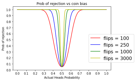
def plot_powers(ax):
ax.set_title("Prob of rejection vs coin bias")
plot_power(100, ax, color='r', label="flips = 100")
plot_power(250, ax, color='b', label="flips = 250")
plot_power(1000, ax, color='g', label="flips = 1000")
plot_power(3000, ax, color='y', label="flips = 3000")
ax.legend(bbox_to_anchor=(0.75, 0.6), loc=2, prop={'size':16})
plot_powers(ax)
Let’s zoom in
fig, ax = plt.subplots(1, 1)
plot_powers(ax)
ax.annotate('Power > 0.9', xy=(0.4758, 0.95), size=16)
ax.fill_between([0, 1.0], [0.9, 0.9], [1.0, 1.0], alpha=0.2)
ax.set_ybound((0.85, 1.01))
ax.set_xbound((0.3, 0.7))
ax.set_xticks(np.arange(0.30,0.70,0.04));
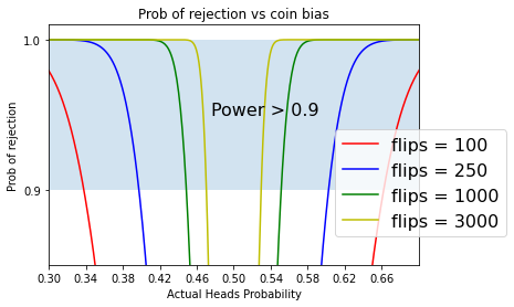
If we only flipped 100 times, then in order for our test to have 90% power the bias of the coins would need to be $p < 0.34$ or $ p>0.66$
If we however flipped 1000 times, then for the same power if the bias is $p<0.45$ or $p > 55$
With 100 flips, we can only distinguish a very bias coin where p<0.34p<0.34 or p>0.66p>0.66 from a fair coin 90% of the time. With 10 times more flips (1000), we can distinguish a less bias coin where p<0.45p<0.45 or p>0.55p>0.55 from a fair coin 90% of the time.
We need a big sample size if we are going to detect small deviations from a fair coin with reasonable power.
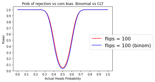
Exact analysis given flips follow a binomial distribution
from scipy.stats import binom

def binom_coin_reject(n, p, alpha=0.05):
    """We can also do this binomial instead of CLT and standard normals
    """
    # confidence interval for p = 0.5 for n flips
    lower, upper = binom.interval(1 - alpha, n, 0.5)
    return 1 - (binom.cdf(upper, n, p) - binom.cdf(lower - 1, n, p))


fig, ax = plt.subplots(1, 1)
ax.set_title("Binomial prob of reject vs coin bias for n = 100")

def plot_binomial_power(n, ax, **kwargs):
    p_values = np.linspace(0,1,1000)
    ax.plot(p_values, binom_coin_reject(n, p_values), **kwargs)
    ax.set_xticks(np.arange(0,1.1, 0.1))
    ax.set_yticks(np.arange(0,1.1, 0.1))
    ax.set_ybound((0, 1.05))
    ax.set_ylabel("Power")
    ax.set_xlabel("Actual Heads Probability")


fig, ax = plt.subplots(1, 1)

def plot_comparison(ax):
    ax.set_title("Prob of rejection vs coin bias. Binomial vs CLT")
    plot_power(100, ax, color='r', label="flips = 100")
    plot_binomial_power(100, ax, color='b', label="flips = 100 (binom)")
    ax.legend(bbox_to_anchor=(0.75, 0.6), loc=2, prop={'size':16})

plot_comparison(ax)
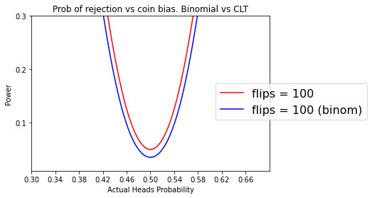
Zooming in
fig, ax = plt.subplots(1, 1)
plot_comparison(ax)
ax.set_ybound((0.01, 0.3))
ax.set_xbound((0.3, 0.7))
ax.set_xticks(np.arange(0.30,0.70,0.04));
If we did the same thing but with $n=1000$
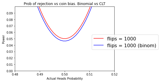


Comments