The Delta Method

The Delta Method

Review of the CLT

If we have some random variables $X_1, \dots, X_n$, which are all i.i.d (independent and identically distributed), and have a common population mean $\mu$, and population variance $\sigma^2$, and we consider the sample mean

\[\bar{X}_n = \frac{1}{n} \sum_{i=1}^n X_i\]

The Central Limit Theorem (CLT) tells us that the sum of those variables, and therefore the sample mean will tend to a Gaussian random variable as $n \to \infty$,

\[\bar{X}_n \stackrel{(d)}{\to} \mathcal{N}\]

Let’s consider the expectation of this sample mean. By linearity of expectation (the expectation of the sum is the sum of the expectations)

\[\mathbb{E}(\bar{X}_n)=\frac{1}{n}\sum_{i=1}^n \mathbb{E}(X_i)\]

and by i.i.d (same distribution in particular)

\[\mathbb{E}(\bar{X}_n)=\frac{1}{n}n \times \mathbb{E}(X_1)= \mathbb{E}(X_1) = \mu\]

Note, it’s important here to distinguish the population mean — the true mean of the underlying distribution that these variables are sampling, and the sample mean. The former is just a scalar constant, and the latter is itself a random variable, that will vary per experiment, and depend on what observations we made that time.

The law of large numbers (LLN) guarantees however that the sample mean will converge to $\mu$ as $n \to \infty$.

Similarly, consider the variance of the sample mean

\[\text{var}(\bar{X}_n)=\text{var}\left(\frac{1}{n}\sum_{i=1}^n X_i\right)\]

Now using independence and $\text{var}(aX+bY)=a^2\text{var}(X) + b^2\text{var}(Y)$

\[\begin{aligned} \text{var}(\bar{X}_n)&=\frac{1}{n^2}\sum_{i=1}^n \text{var}(X_i)\\ &=\frac{1}{n^2}\times n \times \text{var}(X_1)\\ &=\frac{\sigma^2}{n} \end{aligned}\]

So if we take our $\bar{X}_n$ remove its mean and rescale by the square-root of its variance, we will have convergence (in distribution) to a standard Gaussian as $n \to \infty$

\[Z_n = \frac{\bar{X}_n - \mu}{\sqrt{\sigma^2/n}} \xrightarrow[n \to \infty]{(d)} \mathcal{N}(0, 1)\]

(Note the square root is there because $\text{var}(aX)=a^2\text{var}(X)$, so the constant in the denominator will end up being squared, and things all work out to ensure $Z_n$ has a variance of $1$, as is easy to check.

What about a function of my random variable?

Generally if I have some sequence of random variables $(X_n)_{n\ge1}$ (these could be my sequence of sample means as the sample size gets larger and larger for example), such that

\[\sqrt{n}(X_n - \theta) \xrightarrow[n \to \infty]{(d)} \mathcal{N}(0, \sigma^2)\]

for some $\theta \in \mathbb{R}, \sigma^2 \in \mathbb{R}$

Then

\[\sqrt{n}(g(X_n) - g(\theta)) \xrightarrow[n \to \infty]{(d)} \mathcal{N}(0, \sigma^2\cdot[g'(\theta)]^2)\]

where $g$ is some differentiable function at $\theta$

Proof

Using the mean value theorem, if $z>\theta$, then we know there is a number $c_z$ between $z$ and $\theta$, such that

\[g'(c_z) = \frac{g(z)-g(\theta)}{z - \theta}\]

which can also be written as

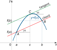
\[g(z) = g(\theta) + g'(c_z)(z-\theta)\]

Hopefully this image provides some geometric intuition for the mean value theorem

It’s really just saying that if a function connects 2 points, then at some point(s) between them the gradient of that function will have to equal the gradient of the straight line connecting those points. It doesn’t tell us what that point is, only that it must exist.

Similarly if $z<\theta$

\[\begin{aligned} g(z) &= g(\theta)-g'(c_z)(\theta-z) \\ &= g(\theta)+g'(c_z)(z-\theta) \end{aligned}\]

i.e. the same form holds and generally we can say $

c_z-\theta

<

z-\theta

$

Now for a random variable $Z$

\[g(Z)-g(\theta)=g'(c_Z)(Z-\theta)\,\,\, ,\text{for some} \,\,|c_Z-\theta|<|Z-\theta|\]

Now given some sequence $(Z_n)_{n\ge 1}$ and any $\mu$, the above statement would be true for any value in the sequence

\[g(Z_n)-g(\mu)=g'(c_{Z_n})(Z_n-\mu)\,\,\, ,\text{for some} \,\,|c_{Z_n}-\mu|<|Z_n-\mu|\]

Applying this to the sample mean. $X_1, \dots, X_n \stackrel{iid}{\sim} X$ and $\mathbb{E}(X)=\mu$, then

\[\sqrt{n}(g(\bar{X_n})-g(\mu))=g'(C_{\bar{X}_n})\left(\sqrt{n}(\bar{X}_n-\mu)\right)\,\,,\text{with}\,\,\,|c_{\bar{X}_n} - \mu| < |\bar{X}_n - \mu|\]

But now by the CLT, we know that the 2nd factor on the right is asymptotically normal

\[\sqrt{n}(\bar{X}_n - \mu) \xrightarrow[n \to \infty]{(d)} \mathcal{N}(0, \sigma^2)\]

Now also notice that by the law of large numbers

\[\bar{X}_n \xrightarrow[n \to \infty]{\mathbb{P}} \mu\]

That means that $\bar{X}n$ and $\mu$ are being squeezed together, and it also means that the number $c{\bar{X}_n}$ is going to head toward $\mu$ as $n$ gets larger and larger. More formally, we could make an argument in convergence of probability. Since

\[|C_{\bar{X}_n}-\mu| < \left|\bar{X}_n - \mu \right|\]

then

\[\mathbb{P}\left(|C_{\bar{X}_n}-\mu| > \epsilon \right) < \mathbb{P}\left(|\bar{X}_n-\mu| > \epsilon \right)\]

and given

\[\bar{X}_n \xrightarrow[n \to \infty]{\mathbb{P}} \mu\]

this implies

\[\lim_{n\to\infty} \mathbb{P}\left(|C_{\bar{X}_n}-\mu|\right) =0\]

which tells us that $C_{\bar{X}_n}$ converges to $\mu$ in probability

\[C_{\bar{X}_n} \xrightarrow[n \to \infty]{\mathbb{P}} \mu\]

The Continuous Mapping Theorem tells us that continuous functions preserve the limits, and $g’$ is by assumption continuous, so we can write

\[g(C_{\bar{X}_n}) \xrightarrow[n \to \infty]{\mathbb{P}} g(\mu)\]

So let’s recap, on the right-hand side we have 2 factors, and for each we have established some convergence

We had originally,

\[g'(C_{\bar{X}_n})\left(\sqrt{n}(\bar{X}_n-\mu)\right)\]

and we’ve found that individually the factors converge as

\[\begin{aligned} g'(C_{\bar{X}_n}) &\xrightarrow[n \to \infty]{\mathbb{P}} g'(\mu)\\ \sqrt{n}(\bar{X}_n - \mu) &\xrightarrow[n \to \infty]{(d)} \mathcal{N}(0, \sigma^2) \end{aligned}\]

How does their product converge? Enter Slutsky’s theorem, which says that if some sequence of random variables $X_n$ converge in distribution to $X$, and some other sequence of random variables $Y_n$ converge in probability to a constant $c$, then $X_n Y_n$ converges *in distribution$ to $X\times c$.

In other words, we are allowed to do the simple thing, and just multiply the limits of our factors together.

So that’s it, we’re done…putting this all together we find

\[\begin{aligned} \sqrt{n}(g(\bar{X_n})-g(\mu)) &\xrightarrow[n \to \infty]{(\mathbb{d})} g'(\mu)\mathcal{N}(0, \sigma^2)\\ &\xrightarrow[n \to \infty]{(\mathbb{d})}\mathcal{N}(0, \left( g'(\mu)\right)^2\sigma^2)\\ \end{aligned}\]

Where the final step follows from $\text{var}(aX)=a^2\text{var}(X)$, i.e. multiplying the distribution by a constant, leaves its mean unchanged and changes the variance to the constant squared times the original variance.

That’s it for the univariate (one variable) version of the delta method. Stay tuned for the multivariate version coming soon.