A/B Tests and Experiment Size

Let’s say you’re running an A/B test. Maybe you want to test how many conversions you will get if you change the design of the Signup page or the wording. You split users landing on your site into 2 groups - the control group and the experimental group. Those in the control group see the existing site and those in the experimental group see the new design. Practically you could do this by setting a cookie or otherwise.

If your baseline rate (the current number of conversions) is 10%, and you wish to be sensitive to an effect size of just 2% (i.e. an increase from 10% to 12%), one question you should ask is how many observations must I make such that my test has a given level and power.

Refresher

Before we dive into answering this question, it is useful to review the concepts of level and power.

Level and Type I error

The level specifies our tolerance for Type I error. That is to say when we reject the null hypothesis when we should not; we reject the null hypothesis when it is in fact true. This is like the percentage of the time we convict an innocent person or the percentage of time when we conclude a placebo is effective.

Another way to see it is to imagine our experiment is coin tossing and we wish to know if the coin is fair (50% probability of heads) or if it is biased (>50% chance of heads). Even with a fair coin, there is some probability that we get an extreme result, say we get 750/1000 heads, despite the coin being fair, just by pure variance.

If we have a level $\alpha=0.05$, which is the common value taken, then only 5% of the time do we commit Type I error.

Power and Type II

Type II error is, on the other hand, when we should reject the null hypothesis but we fail to.

For example, if the coin has 52% of heads it is very likely to not produce an extreme result and we are unlikely to be able to get an extreme enough (given a level of 5%) result for us to be able to reject the null hypothesis that the coin is fair. Intuitively our study would need to include a huge number of coin tosses to stand any chance of being able to conclude the coin is biased and reject the null.

Usually, we write $\beta%$ for the percentage of the time we commit Type II, failing to reject the null hypothesis when we should.

Power is related to this as $1-\beta$. It’s the percentage of the time we correctly reject the null hypothesis. It’s the probability of avoiding committing a Type II error.

A common value for power is 80%.

Experiment size

The question we want to answer is given a desired level and power for our study, and given an effect size we wish to be sensitive to, what is the minimum number of observations we need to make?

Test statistic and power

Let’s say we collected data from the study described above:

condition	signup
1	0
0	0
0	0
1	1

The “condition” just tells us if the user was in the control or experimental groups (0 means control, 1 means experimental). The “signup” column tells us if the ultimately signed up or not.

The null hypothesis is that the new design has no effect on signups and the alternative hypothesis is that the new design caused a bump in signups.

Each observation is a Bernoulli trial taking on 0 or 1 with some probability $p$. Recall that the mean of such a random variable is $p$ and the variance is $p(1-p)$.

We know from the CLT that if we sum up random variables then the resulting random variable will be normally distributed.

Let,

\[\bar{X}_E=\frac{1}{n_E}\sum_i^{n_E} X_E\]

specify the mean of the experimental group signups, and let

\[\bar{X}_C=\frac{1}{n_C}\sum_i^{n_C} X_C\]

be the mean of the control group signups.

Furthermore, let

\[Y = \bar{X}_E - \bar{X}_C\]

In order to standardize, let’s compute the variance of $Y$:

\[\begin{aligned} \text{var}(Y) &= \text{var}(\bar{X}_E - \bar{X}_C)\\ & = \text{var}(\bar{X}_E) + (-1)^2 \text{va}(\bar{X}_C)\\ & = \text{var}(\bar{X}_E) + \text{va}(\bar{X}_C)\\ & = \frac{1}{n_E^2}\times n_E \times \text{var}(X_E) + \frac{1}{n_C^2}\times n_C \times \text{var}(X_C)\\ &=\frac{1}{n_E} p_E(1-p_E) + \frac{1}{n_C}p_C(1-p_C)\\ \end{aligned}\]

Now under the null hypothesis the mean of $Y$ is $\mu_Y=0$, and

\[\text{var}(Y)_{H_0}=p_C(1-p_C)\left[\frac{1}{n_E} + \frac{1}{n_C}\right]\]

whereas under the alternative hypothesis the mean is the effect size (e.g. 0.02 in the example above) and the variance is

\[\text{var}(Y)_{H_1}=\frac{1}{n_E} p_E(1-p_E) + \frac{1}{n_C}p_C(1-p_C)\]

If we designed our study with the test-statistic

\[T_n = \frac{\bar{X}_E - \bar{X}_C}{\sqrt{\text{var}(Y)_{H_0}}}\]

The under the null-hypothesis we know that $T_n$ would follow the standard normal distribution $\mathcal{N}(0, 1)$, and we’d use a one-sided test. To ensure a level $\alpha=0.05$ we would demand that

\[P(T_n > q_{critical}) = 0.05\]

and find $q_{critical} = q_{1-\alpha}$, being the $1-\alpha$ quantile.

We will reject the null hypothesis whenever $T_n$ exceeds that critical value.

However, under the alternative hypothesis the mean of $T_n$ would be $(p_{alt}- p_{null} )/\sqrt{\text{var}(Y)_{H_0}}$, and the standard deviation would be

\[\sqrt{\text{var}(Y)_{H_1}/\text{var}(Y)_{H_0}}\]

Thus one way we can compute the power is just looking for the probability that under the alternative hypothesis our test-statistic falls below the critical value.

def power(p_null, p_alt, n1, n2, alpha = .05, plot = True):
    """
    Compute the power of detecting the difference in two populations with 
    different proportion parameters, given a desired alpha rate.
    
    Input parameters:
        p_null: base success rate under null hypothesis
        p_alt : desired success rate to be detected, must be larger than
                p_null
        n1     : number of observations made in first group
        n1     : number of observations made in second group
        alpha : Type-I error rate
        plot  : boolean for whether or not a plot of distributions will be
                created
    
    Output value:
        power : Power to detect the desired difference, under the null.
    """
    # Compute the power

    # Under the null T_n follows a standard normal by design
    null_dist = stats.norm(loc=0, scale=1)
    p_crit = null_dist.ppf(0.95)
    
    # Under the alt we compute the mean and stddev of the normal disitribution T_n would follow
    se_null = np.sqrt(p_null * (1-p_null) * (1/n1 + 1/n2))
    se_alt = np.sqrt(((p_null * (1-p_null))/n1) + ((p_alt * (1-p_alt))/n2))
    alt_dist = stats.norm(loc=(p_alt-p_null)*(1/se_null), scale=se_alt/se_null)

    # Beta (the probability of committing Type II) is the probability that our alt distribution is below critical
    # and thus we fail to reject (when we should!)
    beta = alt_dist.cdf(p_crit)
    
    # Display a nice plot
    if plot:
        # Compute distribution heights
        low_bound = null_dist.ppf(.01)
        high_bound = alt_dist.ppf(.99)
        x = np.linspace(low_bound, high_bound, 201)
        y_null = null_dist.pdf(x)
        y_alt = alt_dist.pdf(x)

        # Plot the distributions
        plt.plot(x, y_null)
        plt.plot(x, y_alt)
        plt.vlines(p_crit, 0, np.amax([null_dist.pdf(p_crit), alt_dist.pdf(p_crit)]),
                   linestyles = '--')
        plt.fill_between(x, y_null, 0, where = (x >= p_crit), alpha = .5)
        plt.fill_between(x, y_alt , 0, where = (x <= p_crit), alpha = .5)
        
        plt.legend(['null','alt'])
        plt.xlabel('difference')
        plt.ylabel('density')
        plt.show()
    
    # return power
    return f'The power is {(1 - beta)*100: .2f}%'

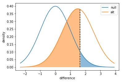
As an example, we see that with an effect of 10%-12% and a level of 5%, even with 1000 observations (500 in each group), we have a power of just 44%. That means we have only a 44% chance of actually being able to reject the null and pick up the increased signups.

Computing the experiment size analytically

If both $\alpha$ and $\beta$ are less than 50% (which in practice is always going to be the case), the critical value will fall between zero and the mean of the test-statistic under the alternative hypothesis.

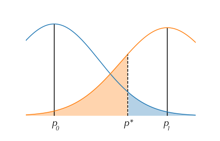
We know the critical value is $q_{1-\alpha}$, which is the $1-\alpha$ quantile.

Under the alternative hypothesis the distribution of $T_n$ has mean

\[\mu_{alt} = \frac{p_{alt}- p_{null}}{\sqrt{\text{var}(Y)_{H_0}}}\]

and

\[\mu_{alt} - q_{1-\alpha} = -q_{\beta} \times \sqrt{\text{var}(Y)_{H_1}/\text{var}(Y)_{H_0}}\]

because the alternative distribution has a variance that is not $1$, the quantile is multiplied by that variance. As you can verify by considering

stats.norm(loc=0, scale=16).ppf(0.95)/stats.norm(loc=0, scale=1).ppf(0.95)
>>> 16

Plugging in

\[\frac{p_{alt}- p_{null}}{\sqrt{\text{var}(Y)_{H_0}}} - q_{1-\alpha} = -q_{\beta} \times \sqrt{\text{var}(Y)_{H_1}/\text{var}(Y)_{H_0}}\]

After some algebra

\[p_{alt}- p_{null} = q_{1-\alpha}{\sqrt{\text{var}(Y)_{H_0}}} -q_{\beta} \times \sqrt{\text{var}(Y)_{H_1}}\]

For simplicity assume that $n_E=n_C=n$, so that

\[\sqrt{\text{var}(Y)_{H_0}} = \frac{\sqrt{2 p_C(1-p_C)}}{\sqrt{n}}\]

and

\[\sqrt{\text{var}(Y)_{H_1}} = \frac{\sqrt{p_E(1-p_E) + p_C(1-p_C)}}{\sqrt{n}}\]

Then we have

\[p_{alt}- p_{null} = q_{1-\alpha}\frac{\sqrt{2 p_C(1-p_C)}}{\sqrt{n}} -q_{\beta} \frac{\sqrt{p_E(1-p_E) + p_C(1-p_C)}}{\sqrt{n}}\]

Solving for $n$:

\[n = \left[\frac{q_{1-\alpha}\sqrt{2 p_C(1-p_C)} - q_{\beta}\sqrt{p_E(1-p_E) + p_C(1-p_C)}}{p_{alt}- p_{null} }\right]^2\]

def experiment_size(p_null, p_alt, alpha = .05, beta = .20):
    """
    Compute the minimum number of samples needed to achieve a desired power
    level for a given effect size.
    
    Input parameters:
        p_null: base success rate under null hypothesis
        p_alt : desired success rate to be detected
        alpha : Type-I error rate
        beta  : Type-II error rate
    
    Output value:
        n : Number of samples required for each group to obtain desired power
    """
    
    # Get necessary z-scores and standard deviations (@ 1 obs per group)
    z_null = stats.norm.ppf(1 - alpha)
    z_alt  = stats.norm.ppf(beta)
    sd_null = np.sqrt(p_null * (1-p_null) + p_null * (1-p_null))
    sd_alt  = np.sqrt(p_null * (1-p_null) + p_alt  * (1-p_alt) )
    
    # Compute and return minimum sample size
    p_diff = p_alt - p_null
    n = ((z_null*sd_null - z_alt*sd_alt) / p_diff) ** 2
    return np.ceil(n)

This can also be computed using tools such as this

It can also be computed using the statsmodels python lib:

# example of using statsmodels for sample size calculation
from statsmodels.stats.power import NormalIndPower
from statsmodels.stats.proportion import proportion_effectsize

# leave out the "nobs" parameter to solve for it
NormalIndPower().solve_power(effect_size = proportion_effectsize(.12, .1), alpha = .05, power = 0.8,
                             alternative = 'larger')