Logistic Regression from scratch

3 minute read

Logistic unit

In simple Logistic Regression, we have the cost function

$\mathcal{L}(a, y) = -yln{(a)} - (1-y)ln{(1-a)}$

whereb $a$ is the predicted value and $y$ is the ground-truth label on the training set ( ${0, 1}$ ).

Why this function? The intuitive version is that if $y=1$ the second term goes away, and the first term that remains is small when $a\to 1$ (i.e. the predicted value approaches the correct ground truth), yet large when $a\to 0$ (i.e. we are punished with a large cost when the predicted answer goes away from the ground truth). Similarly for the other term.

Stats asidePermalink

However, the more mathemtically rigorous answer is that this function comes from the MLE (Maximum Likelihood Estimator). Recall that if we have a Bernoulli model, then we can write

$L(x_1, \dots, x_n; p) = p^{\sum_{i=1}^{n} x_i}(1-p)^{n-\sum_{i=1}^{n} x_i}$

Recall we want the argmax over $p$ of this function, but since the logarithm is monatonically increasing this amounts to the same as finding the max over the log-likelihood

$\mathcal{l} = \log{L(x_1, \dots, x_n; p)} = \left(\sum_{i=1}^{n} x_i\right) \log{p} + \left(n-\sum_{i=1}^{n} x_i\right)\log({1-p})$

In regular statistics class, we’d now find the maxima by taking deratives and setting equal to 0. This would give us the MLE estimator of our paramter $p$ , which not too surprisngly would turn out to be the average

$p^{\text{MLE}} = \frac{1}{n}\sum_{i=1}^n x_i$

For a single training example the log-likelihood would be

$\mathcal{l}_1 = x \log{p} + \left(1-x\right)\log({1-p})$

and we not that finding the maxima of this function is equivalent to finding the minima of the negative. With a small change of notation, we see the negative is exactly our usual logistic regression cost function.

Back to MLPermalink

BackpropPermalink

We will need to know how our cost-function varies as our network weights vary. To that end let’s compute a few things

$\frac{\partial\mathcal{L}}{\partial a} = -\frac{y}{a}+\frac{(1-y)}{(1-a)}$

Then we also used the sigmoid activation function

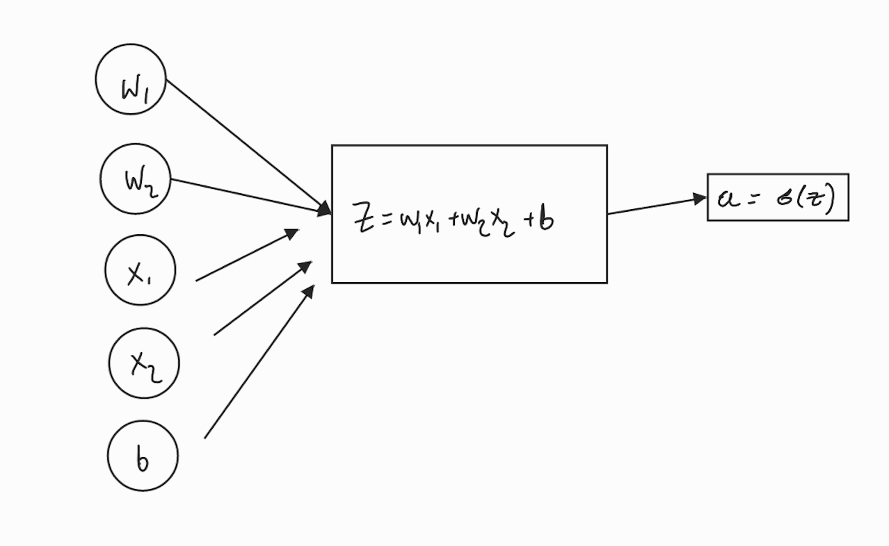
$a = \sigma(z) = \frac{1}{1+e^{-z}}$

meaning

$\begin{aligned} \frac{da}{dz} &= \frac{e^{-z}}{(1+e^{-z})^2} \\ &=\frac{1}{1+e^{-z}}\frac{1+e^{-z}-1}{1+e^{-z}} \\ &=a(1-a) \\ \end{aligned}$

Now we can simply use the chain rule to get the dependence on $z$ :

$\begin{aligned} \frac{d\mathcal{L}}{dz} &= \frac{\partial \mathcal{L}}{\partial a}\frac{\partial a}{\partial z} \\ &=a(1-a)\left[-\frac{y}{a}+\frac{(1-y)}{(1-a)}\right] \\ &= -y(1-a) + a(1-y) \\ &= a-y \end{aligned}$

The final step

Given that $z$ depends on the network’s weights $w_1, w_2, b$ and the training features, $x_1, x_2$ as follows

$z = w_1 x_1 + w_2 x_2 + b$

and

$\frac{dz}{dw_i} = x_i$

and

$\frac{dz}{db} = 1$

Applying the chain-rule just one more time and we get the final result

$dw_i = \frac{d\mathcal{L}}{dw_i} = x_i (a-y)$

and

$db = \frac{d\mathcal{L}}{db} = (a-y)$

Gradient descent update rulePermalink

So to perform gradfient descent we must update our parameters as follows:

$\begin{aligned} w_1 & = w_1 - \alpha dw_1 \\ w_2 & = w_2 - \alpha dw_2 \\ b & = b - \alpha db \\ \end{aligned}$

where $\alpha$ is the learning rate and controls the size of the steps we take.

Vectorizing Logistic RegressionPermalink

So for the i’th training example, the forward step would look like

$\begin{aligned} z^{(i)} &= w^{T}x^{(i)} + b\\ a^{(i)} &= \sigma(z({i})) \end{aligned}$

so for $m$ training examples we’d traditionally have a for loop iterating over each. However this is inefficient.

Consider the design matrix $X$ :

$\mathbf{X}=\begin{pmatrix} \vert & \dots & \vert \\ x^{(1)} & \dots & x^{(m)} \\ \vert & \dots & \vert \end{pmatrix}$

This is an $n \times m$ matrix, where we have $m$ training examples and $n$ features.

Using this matrix, we can do the forward step over all examples at once

$[z^{(1)}, z^{(2)}, \dots, z^{(m)}] = w^{T} X + [b,b, \dots, b]$

$Z = w^{(T)} X + b$

or in code

# Note: python will broadcast the scalar b 
Z = np.dot(w.T, X) + b

Gradient computationPermalink

$dz^{(i)} = a^{(i)} - y^{(i)}$

and we define the $1\times m$ ector

$dZ = [dz^{(1)}, \dots, dz^{(m)}]$

so vectorizing our computation, and with similar definitions for the vectors $A$ and $Y$ , we’d have

$dZ = A - Y$

We had

$db = \frac{1}{m} \sum_1^m z^{(i)}$

which translates to

db = np.sum(dZ)/m

and

$dw = \frac{1}{m} X dZ^{(T)}$

expanding this

$\begin{aligned} dw &= \frac{1}{m} \begin{pmatrix} \vert & \dots & \vert \\ x^{(1)} & \dots & x^{(m)} \\ \vert & \dots & \vert \end{pmatrix} \begin{pmatrix} dz^{(1)} \\ \dots \\ dz^{(m)} \end{pmatrix} \\ & = \frac{1}{m}\left[x^{(1)} dz^{(1)} + \dots + x^{(m)}dz^{(m)}] \end{aligned}$

Note that here the resulting $dw$ is an $n\times 1$ vector.

In code and altogether

Z = np.dot(W.T, X) + b
A = sigma (Z)
dZ = A - Y
dw = (1/m) np.dot(X, dZ.T)
db = 1/m np.sum(dZ)

Then the gradient ascent update goes as

w = w - alpha dw
b = b - alpha db

We still need an outer for-loop over all the iterations of gradient ascent, but aside that we have vectorized all that is possible.

Whatsapp Twitter Facebook LinkedIn

Lee H

Logistic Regression from scratch

Stats asidePermalink

Back to MLPermalink

BackpropPermalink

Gradient descent update rulePermalink

Vectorizing Logistic RegressionPermalink

Gradient computationPermalink

Comments

You May Also Enjoy

A/B Tests and Experiment Size

NLP Pipelines with NLTK

Useful Pandas Snippets

Deploying imgproxy with AWS Fargate